No-fee trading has invited a huge influx of people new to trading. In this article, I will discuss the basics of “price formation”, the mechanism by which stock prices are determined.
Like most people, for much of my life I assumed that every stock has a well-defined “price” at any given point in time. You could buy or sell at that price, and the price would move based on activity. If it went up you made money, if it went down you lost money. Trading was easy: you just bought the stocks you thought would go up and sold the ones you thought would go down.
Unfortunately, my blissful naivete was cut short. After a youthful indiscretion, I ended up doing five years at the Massachusetts Institute of Technology. When the doors finally slammed shut behind me, I emerged with little more than a bus ticket and some physics-department issued clothes. Nobody reputable would hire a man with a checkered background doing physics, so I ended up with the only sort open to hard cases: Wall Street.
I caught the eye of a particularly unsavory boss one day, and he recruited me into a gang doing stat arb at a place called Morgan Stanley. I tried to get out, but they kept pulling me back in. It took six years to find a way out, but even then freedom proved elusive. I was in and out of corporations for the next few years, and even did some contract work for a couple of big hedge funds. Only in the confusion of 2008, did I finally manage to cut ties and run. But the scars are still there. The scars never go away.
On the plus side, I did learn a bit about market microstructure. Along the way I came to understand that my original view of prices was laughably simplistic. My hope is that I can help some misguided kid somewhere avoid my own missteps. If I can save even one reader, the effort put into this post will have been repaid a thousand times over. Mainly because I didn’t put much effort into it.
Rather than a detailed exposition on market microstructure (which varies from exchange to exchange, but has certain basic principles), I will go through a number of possible misconceptions. Hopefully, this will be of some small help to new traders who wish to better understand the dynamics of the stock market. At the very least, it will make you sound smart at cocktail parties. It also may help the occasional reader avoid such minor faux pas as redditing “hey guys, why don’t we all collude to manipulate stock prices in clear violation of SEC regulations, and to such an absurd degree that it will be impossible for regulators NOT to crucify us.” But hey, what’s the worst that could result from the public subversion of a number of powerful, well-connected hedge funds and the defiant proclamation that this was intentional?
Now to the important bit. Because we live in America, and everybody sues everyone for everything, I’ll state the obvious. Before you do anything, make sure you know what you are doing. If you read it here, that doesn’t mean it’s right or current. Yes, I worked in high frequency statistical arbitrage for some time. However, my specific knowledge may be dated. Though the general principles I describe still apply, you should confirm anything I say before relying heavily on it. In particular, I am no tax expert. Be sure to consult an accountant, a lawyer, a doctor, a rabbi, and a plumber before attempting anything significant. And if you do, please send me their info. It’s really hard to find a good accountant, lawyer, doctor, rabbi, or plumber.
Don’t take anything I say (or anyone else says) as gospel. I’ve tried to be as accurate as possible, but that doesn’t mean there aren’t technical errors. As always, the onus is on you to take care of your own money. When I first started out on Wall Street, I was in awe of traders. Then I got to know some. In my first job, somebody helpfully explained why people on Wall Street were paid more than in other professions. They weren’t paid to be infallible and never make mistakes; they were paid to be attentive and diligent enough to catch any mistakes they did make.
This sounded nice, but turned out to be a load of malarkey. The highly-paid professionals on Wall Street are the same bunch of knuckleheads as in any other profession, but with better credentials. However, this cuts both ways. Many people have a view, promulgated by movies and television, that bankers are unscrupulous, boiler-room shysters. These certainly exist, but mostly amongst the armies of low-paid retail brokers, or in certain very disreputable areas such as commercial banking. The real Wall Street is quite different. The individuals I worked with were highly ethical, and the environment was far more collegial and honest than academia. And this was in the late 90’s and early 2000’s, before academia really went to pot. The few knives I had to pull out of my back were (with one exception) gleefully inserted by fellow former-physicists. Fortunately, while physicists know a lot about the kinematics of knives, they know very little about anatomy. I emerged unscathed, and even got a few free knives out of it — which I promptly sold to some folks in Academia, where such things always are in high demand.
Despite its inapplicability to actual employee behavior, the point about mistakes is a good one. It is impossible to avoid making mistakes, but if you value your money you should carefully triple-check everything. This goes doubly for any work done by an accountant, financial adviser, or other “professional” you ill-advisedly employ. They probably know less than you do, and certainly care less than you do about your money.
The best advice I can offer is to inform yourself and be careful. Do research, check, recheck, and recheck again before committing to a trade. In my personal trading, I’ve never lost out by being too slow or cautious. But I have been hammered by being too hasty.
Now to the possible misconceptions. I’ll call them “myths” because that’s what popular websites do, so obviously it’s the right thing to do, and I prefer to do the right thing because the wrong thing rarely works.
Myth 1: There is a “price” for a stock at any given point in time. When a stock is traded during market hours, there is no such thing as its “price”. There is a bid (the highest offer to buy) and an ask (the lowest offer to sell). Often, the “price” people refer to is the last trade price (the price at which the last actual transaction occurred, regardless of its size). Sometimes the midpoint (bid+ask)/2 or weighted midpoint (bid x bidsize + ask x asksize)/(bidsize + asksize) is used. For algorithmic trading, more complicated limit-book centroids sometimes are computed as well. The “closing price” generally refers to the last trade price of the day. This is what appears in newspapers.
Myth 2: I can place a limit order at any price I want. No, you cannot. Stocks (and options) trade at defined ticks. The “tick” or “tick size” is the space between allowed prices, and may itself vary with price. For example, the tick size in stock ZZZ could be $0.01 for prices below $1.00 and $0.05 otherwise. Often, ticks are things like 1/8 or 1/16 rather than multiples of $0.01. The tick size rules vary per exchange (or per security type on a given exchange) rather than per stock. In our example, any stock’s price could have allowable values of …, $0.98, $0.99, $1.00, $1.05, $1.10, … on the exchange in question.
Myth 3: Limit Orders always are better than market orders. Limit orders offer greater control over the execution price, but they may not be filled or may result in adverse selection. Suppose ZZZ is trading with a bid of $100, an ask of $101, and a tick size of $0.50. Alice places a buy limit order at $100.5. It is quite possible that it quickly will be filled, giving her $0.50 better execution than a market order.
But suppose it is not filled right away. If the stock goes up, Alice has incurred what is called “opportunity cost.” The $0.50 attempted savings now translates into having to pay a higher price or forego ownership of the stock. It’s like waiting for the price of a home to go down, only to see it go up. If you want the home (and still can afford it), you now must pay more.
Ok, but why not just leave the limit order out there indefinitely? Surely it will get filled at some point as the stock bounces around. And if not, there is no harm. You don’t end up with the stock, but haven’t lost any money. In fact, why not put a limit order at $98? If it gets executed, that’s a $2.00 price improvement!
The problem is adverse selection. Such a limit order would get filled when the stock is falling. Sure, a temporary dip could catch it. But a major decline also could. The order is likely to be filled under precisely the conditions when Alice would not want it to be. At that point, she may be able to buy the stock for $97 or $96 — if buying it remains desirable at all. In the presence of an “alpha” (loosely speaking, a statistical signal which a trader believes has some predictive power for future stock movements), it may pay to place such limit orders —but that is a specific execution strategy based on a specific model. In general, there is no free money to be had. You either incur the transaction cost of crossing the spread (i.e. paying the ask), or risk both the opportunity cost of losing out on a desirable trade and the possibility of adverse selection which lands you with the stock at the worst possible time.
Well, it isn’t strictly true there is no free money to be had. There is free money to be made, but only by market makers, uniquely positioned to accept large volumes of orders. In this, they are not unlike the exchanges themselves. You and I do not possess the technology, capital, or customer flow to make money that way.
Myth 4: I can buy or sell any quantity at the stated price. There are a couple of reasons this is not true. The “stated price” usually is the last trade price, and there is no guarantee you can buy at that same price. Just because a house down the block sold for X doesn’t mean you can buy an identical one now for X. In illiquid stocks (and quite often with options), the last trade may have taken place some time ago and be stale relative to the current quote.
In principle, you can buy at the current ask or sell at the current bid. However, even this is not guaranteed. The bid and ask can move quickly, and it may be difficult to catch them. But there also is another critical issue at play. The bid and ask are not for unlimited quantities of stock. Each has an associated size, the total number of shares being sold or sought at that price. To understand this, it is necessary to explain how an order actually is executed — and that requires the notion of a “limit book” (aka “order book”).
Most data vendors and websites will display a “quote” (aka “composite quote”) for each stock. This consists of a bid, an ask, a bid-size, and an ask-size. Although some websites may omit the sizes, they are considered part of the quote. Suppose the quote for ZZZ has a bid of $100 for 200 shares, an ask of $101 for 50 shares, and the relevant tick-size is $0.50. Then the spread is two ticks (101-100)/0.50, and the midpoint is $100.50. It isn’t necessarily the case that there is one trader offering to buy 200 shares at $100 and another offering to sell 50 shares at $101. The sizes may be aggregates of multiple orders at those price levels.
The composite quote actually is a window into a larger constellation of orders known as the limit book. The limit book consists of a set of orders at various price levels. For example, the limit book for ZZZ could have orders at $101, $101.5, $102, and $104 on the ask side, with a queue of specific orders at each level. The composite quote simply is the highest bid, the lowest ask, and the aggregate size for each.
Suppose Bob puts in a market order to buy $100 shares of ZZZ. This is matched against the orders at the lowest ask level ($101 in this case) in their order of priority (usually the time-order in which they were received). Since there only are 50 shares at $101, the exchange matches Bob against all the sell-orders at $101. It then matches the remaining 50 shares against the second ask level ($101.5) and higher until it matches them all. If it fails to match them all, Bob will have a partial fill, and the remainder of the order will be cancelled (since it was a market order). Each “fill” is a match against a specific sell-order, and a given trade can result in many fills. This is part of why your broker may sometimes send a bunch of trade confirmations for a single order on your part.
For highly liquid stocks, no order you or I are likely to place will go execute past the inner quote. However, that quote can move quickly and the price at which a market order is executed may not be what you think. Brokers also execute order flow internally, or sell flow to other institutions — which then match it against other customers or their own orders. To you it looks the same (and may actually improve your execution in some cases), but your trade may never make it to the exchange. This is fine, since you’re not a member of the exchange — your broker is.
Note the risk of a market order, especially for illiquid stocks. Suppose the 2nd ask level was $110 rather than $101.5. In that case, Bob would have bought 50 shares at $100 and 50 shares at $110. A limit order slightly past the ask would have avoided this. For example, if he wanted to ensure execution (if possible) but avoid such ridiculous levels, he could place a fill-or-kill (but not all-or-none) order at $102. This would ensure that he doesn’t pay more than $102, but he may only get a partial fill.
For stocks (other than penny-stocks), limit orders rarely are necessary as protection, though they may be desirable for other purposes. But when trading options, a limit order always should be used. If the quote is moving around a lot, this can be a good way to control worst-case execution (but in exchange for some opportunity cost). Options are a bit odd, since brokers often will write them on the spot in response to an order. You just need to figure out what their automated price-level is. Sometimes it is the midpoint, sometimes slightly higher. You almost always can do better than the innermost ask for small volume. For higher volume, you should buy slowly (over a day or two) to avoid moving the market too much — though it may be impossible if you effectively have the broker as your only counterparty. But back to Bob and ZZZ!
Now suppose that Bob places a limit order to buy 50 shares at $100.5, right in the middle of the current spread. There now is a new highest bid level: $100.5, and Bob is the sole order at that level. Any market sell order will match against him first, and this may happen so fast that the quote never noticeably changes. But if not, the new bid and bidsize will be $100.5 and 50 shares. If instead, he placed his buy order at $100, he would join the other bids at $100 as the last in the queue at that level.
What if he places it at $101 instead? If there were 25 shares available at that ask level, he would match those 25 shares. He now would have a bid for the remaining 25 shares at $101. This would be the new best bid, the quote would change accordingly. The new best ask would be $101.5. Finally, suppose he placed the limit order at $110 instead. This effectively would be a market order, and would match against the $101 and $101.5 levels as before. Note that he would not get filled at $110 in this example. If there were 25 shares each at $101 and $101.5, he would be filled at those levels and his $110 limit order would have the same effect as a $101.5 limit order.
The limit book constantly is changing and, to make things worse, there often is hidden size. On many exchanges, it’s quite possible for the limit book to show 25 shares available at $101 and yet fill Bob for all 50 at that level. There could be hidden shares which automatically replenish the sell-order but are not visible in the feed. This is intentional. Most of the time, we only have access to simple data: the current quote and the last trade price.
Note that the crossing procedure described is performed automatically almost everywhere these days. Most exchanges run “ECNs”, electronic crossing networks. An algorithm accepts orders which conform to the tick-size and other exchange rules, crossing them or adjusting the limit book accordingly. This is conceptually simple, but the software is rather involved. Because of the critical nature of an exchange, the technology has to be robust. It must be able to receive high volumes of orders with minimal latency; process them, cross them, and update the limit book; transmit limit-book, quote, and trade information to data customers; manage back-end and regulatory tasks such as clearing trades, reporting them, and processing payments; and do all this at extremely high speed, across many stocks and feeds concurrently, and with significant resilience. It definitely beats a bunch of screaming people and trade slip confetti.
Myth 5: The price at the close of Day 1 is the price at the open of Day 2. This clearly is not true, and often the overnight move is huge and predicated on different dynamics than intra-day moves. There are two effects involved. Some exchanges make provision for after-market and pre-open trading, but the main effect is the opening auction. Whenever there is a gap in trading, the new trading session begins with an opening auction. Orders accumulate prior to this, populating the limit book. However, no fills can occur. This means that the two sides of the limit book can overlap, with some bids higher than some asks. This never happens during regular trading because of the crossing procedure described earlier, and this situation must cleaned up before ordinary trading can begin.
The opening auction is an unambiguous procedure for matching orders until the two sides of the book do not overlap. It is executed automatically by algorithm. The closing price on a given day is the last trade price of that day. It often takes a while for data to trickle in, so this gets adjusted a little after the actual close but usually is fairly stable. The prices one sees at the start of the day involve a flurry of fills from the uncrossing. This may create its own minor chaos, but the majority of the overnight price move is reflected in the orders themselves. Basically, it can be thought of as a queue waiting to get their orders in. There also are certain institutional effects near the open and close because large funds must meet certain portfolio constraints. Note that the opening auction happens any time there is a halt to trading. Most opening auctions are associated with the morning open, but some exchanges (notably the Tokyo Stock Exchange) have a lunch break. Extreme price moves also can trigger a temporary trading halt. In each case, there is an opening auction before trading restarts.
Myth 6: The price fluctuations of a stock reflect market sentiment. That certainly can be a factor, often the dominant one. However, short-term price fluctuations also may be caused by mere market microstructure.
The price we see in most charts and feeds is the last trade price, so let’s go with that. Similar considerations hold for the quote midpoint, bid, ask, or any other choice of “price” that is being tracked.
When you buy at the ask, some or all of the sell-orders at that ask-level of the limit book are filled. There may be hidden size which immediately appears, or someone may happen to jump in (or adjust a higher sell-order down). But in general, this is not the case. The composite quote moves, as do all quote-based metrics. The last trade price also reflects your trade, at least until the next trade occurs.
Consider an unrealistic but illustrative example: ZZZ has a market cap of a billion dollars. Bob and Alice are sitting at home, trading. The rest of the market, including all the major institutions which own stock in ZZZ, are sitting back waiting for some news or simply have no desire to trade ZZZ at that time. They don’t participate in trading, and have no orders outstanding. So it’s just Alice and Bob. ZZZ has a last trade price of $100, Bob has a limit order to buy 1 share at $100, and Alice has a limit order to sell 1 share at $101. These orders form both the quote and the entirety of the limit book (in this case).
Bob gets enthusiastic, and crosses the spread. The price now is $101, that at which his trade transacted. Both see that the “price” just went up, and view the stock as upward-bound. Alice has some more to sell, and decides to raise her ask. She places a sell limit order for 1 share at $102. The ask now is 1x$102. Bob bites, crossing the spread and transacting at $102. The “price” now is $102. The pattern repeats with Alice always increasing the ask by $1 and Bob always biting after a minute or so. The closing price that day $150.
Two people have traded a total of 50 shares over the course of that day. Has the price of a billion dollar company really risen 50%? True, this is a ridiculous example. In reality, the limit book would be heavily populated even if there was little active trading, and other participants wouldn’t sit idly by while these two knuckleheads (well, one knucklehead, since Alice actually does pretty well) go at it. But the concept it illustrates is an important one. Analogous things can happen in other ways. Numerous small traders can push the price of a stock way up, while larger traders don’t participate. In penny stocks, this sort of thing actually can happen (though usually not in such an extreme manner). When a stock’s price changes dramatically, it is important to look at the trading volume and (if possible) who is trading. When such low-volume price moves occur, it is not a foregone conclusion that the price will revert immediately or in the near term. Institutional traders aren’t necessarily skilled or wise, and can get caught up in a frenzy or react to it — so such effects can have real market impact. However, most of the time they tend to be transient.
Myth 7: Shorting is an abstraction, and is just like buying negative shares. In many cases, it effectively behaves like this for the trader. However, the actual process is more complicated. “Naked shorts” generally are not allowed, though they can arise in anomolous circumstances. When you sell short, you are not simply assigned a negative number of shares, which settles accordingly. You are borrowing specific shares of stock from a specific person who has a long position. The matching process is called a “locate” and is conducted at your broker’s level if possible or at the exchange level if the broker has no available candidates. There is an exception for market-makers and for brokers when a stock is deemed “easy to borrow”, meaning it is highly liquid and there will be no problem covering the short if necessary. Brokers maintain dynamic “easy to borrow” and “hard to borrow” lists for this purpose.
From the standpoint of a trader, there are two situations in which a short may not behave as expected. Suppose Bob sells short 100 shares of ZZZ stock, and the broker locates it with Alice. Alice owns 100 shares, and the broker effectively lends these to Bob. If Alice decides to sell her shares, Bob now needs to return the shares he borrowed and be assigned new ones. Normally, this is transparent to Bob. But if replacement shares cannot be located, he must exit his short position. The short sale is contingent on the continuing existence of located shares.
Because of the borrowing aspect, Bob’s broker also must ensure he has sufficient funds to cover any losses as ZZZ rises. This requires a margin. If ZZZ goes up, Bob may have to put up additional capital or exit his position (and take the loss). In principle, a short can result in an unlimited loss. In practice, Bob would fail a margin call before then. I.e., Bob cannot simply “wait out” a loss as he could with a long position.
If — as you should — you view the value of your position as always marked-to-market, then (aside from transaction cost or tax concerns) you never should hold a position just to wait out a loss. Most people don’t think or act this way, and there sometimes are legitimate reasons not to. For example, a long term investment generally shouldn’t be adjusted unless new information arrives (though that information may regard other stocks or externalities which necessitate an overall portfolio adjustment). One could argue that short term random fluctuations do not constitute new information, and without an alpha model one should not trade on them. This is a reasonable view. However, the ability to avoid doing so is not symmetric. Because of the issues mentioned, short positions may be harder to sustain than long ones.
The next couple of myths involve some tax lingo. In what follows “STCG” refers to “Short Term Capital Gain” and “LTCG” refers to “Long Term Capital Gain”. “STCL” and “LTCL” refer to the corresponding losses (i.e. negative gains).
Myth 8: Shares are fungible. When you sell them, it doesn’t matter which ones you sell. This is true from the standpoint of stock trading, but not taxes. Most brokers allow you to specify the specific shares (the “lots”) you wish to sell, though the means of doing so may not be obvious. However, for almost all purposes two main choices suffice: LIFO and FIFO. Most of the time, FIFO is the default. With many brokers, you can change this default for your account, as well as override it for individual trades. Let’s look at the difference between FIFO and LIFO.
Suppose Bob bought 100 shares of ZZZ at $50 3 years ago and bought another 100 shares of ZZZ at $75 6 months ago. ZZZ now is at $100, and he decides to sell 100 shares. If he sells the first 100 shares, a LTCG of $5000 ($10000 – $5000) is generated, but if he sells the second 100 shares a STCG of $2500 ($10000 – $7500) is generated. The implications of such gains can be significant, and are discussed below. The specifics of Bob’s situation will determine which sale is more advantageous — or less disadvantageous.
The first choice corresponds to FIFO accounting: first in, first out. The second corresponds to LIFO: last in, first out. One usually (but not always) benefits from FIFO, which is why this is the default. Note that FIFO and LIFO are relative to a given brokerage account, since a broker only knows what about your positions with it. If Bob had an earlier position with broker B, broker A does not know about it or cannot sell it. In that case, Bob must keep track of these things. FIFO and LIFO are relative to the specific account in question, but the tax consequences for Bob are determined across all brokerage accounts. We’ll see what this means in a moment.
All capital gains are relative to “basis” (or “tax basis”), generally the amount you paid for the stock when you bought it. In the example above, the basis for the first lot was $5000 and the basis for the second was $7500. This was why the LTCG from the first was $5000, while the STCG from the second was $2500. With stocks (but not necessarily mutual funds), a tax event only occurs when you close your position. If you hold the shares for 10 years, only on year 10 is a capital gains tax event generated. This can allow some strategic planning, and part of your overall investment strategy may involve choosing to sell in a low-income year. Note that dividends are taxed when you receive them, and regardless of whether they are cash or stock dividends or you chose to reinvest them. Also note that some mutual funds generate tax events from their own internal trading. You could be taxed on these (STCG or LTCG), and it is best to research the tax consequences of a fund before investing in it.
If you transfer stocks between accounts (usually done when transferring a whole account to a new broker), their tax basis is preserved. No tax events are generated. Note that the transfer must be done right. If you manually close your old positions and open new ones (with enough time between), you may generate a tax event. But if you perform an official “transfer” (usually initiated with your destination broker), the basis is preserved and no tax event occurs. Whether your broker will know that basis is another question. Not every broker’s technology or commitment to customer convenience is up to snuff. It is a good practice to keep your own careful records of all your trading activity.
When would LIFO be preferable? There are various cases, but the most common is to take a STCL to offset STCGs. STCGs tend to be taxed at a much higher rate than LTCGs, so taking a loss against them often is the desirable thing to do. In Bob’s case, if the price had gone down to $25 instead of up to $100, he could sell at a loss and use that loss to offset gains from some other stocks. He would have to specify LIFO to sell the newer lot and generate the STCL.
Myth 9: A “no-fee” trading account is better than one with fees. The cost to a trader involves several components. The main three are broker fees, exchange fees, and “execution”. “No-fee” refers to the broker fee. Unless many small trades are being executed with high frequency, the broker fee tends to be small. The exchange fees are passed along to you, even for “no-fee” accounts. The “execution” is the bulk of the cost. No or low-fee brokers often cross flow internally or sell flow to high-frequency firms which effectively front-run you. Market orders see slightly worse execution than they could, and limit orders get filled with slightly lower frequency than they could (or are deferred, causing slight adverse selection). These effects are not huge, but something to be aware of.
Suppose Alice buys 100 shares of ZZZ at $100. Broker X is no-fee, and Broker Y charges a fee of $7.95 per trade but has 10 bp (0.1%) better execution than Broker X on average. That 10 bp is just a price improvement of $0.10, and amounts to $10. Alice does better with Broker Y than Broker X. This benefit may seem to apply only to large trades, but it also applies to stocks with large spreads. For illiquid stocks (including penny stocks) the price improvement can be much more significant. There are trading styles (lots of small trades in highly liquid stocks) where no-fee sometimes trumps better execution, but most often it does not.
Myth 10: Taxes are something your accountant figures out, and shouldn’t affect your trading. Selling at the best price is all that matters. Taxes can eat a lot of your profit, and should be a primary consideration. Tax planning involves choosing accounts to trade in (401K or other tax-deferred vs regular), realizing losses to offset gains, and choosing assets with low turnover. As mentioned, some mutual funds can generate capital gains through their internal trading. In extreme cases, you could pay significant tax on a losing position in one.
Why are taxes so important to trading? The main reason is that there can be a 25% (or more) difference in tax rate between a LTCG and a STCG. STCGs often are taxed punitively, or at best are treated like ordinary income. Here in MA, the state tax alone is 12% for STCGs vs 5% for LTCGs. Federally, STCGs are treated as ordinary income while LTCGs have their own lower rate.
STCGs are defined as positions held for under one year, while LTCGs are held for over one year. Note that it is the individual positions that matter. If Bob owns 200 shares of ZZZ, bought in two batches, then each batch has its own basis and its own purchase date. Also note that most stock option positions result in a STCG or STCL. A STCG only can be offset by a STCL, but a LTCG can be offset by a LTCL or STCL. Clearly, STCLs are more valuable than LTCLs. They can be rolled to subsequent years under some circumstances, but may be automatically wasted against LTCGs if you are not careful.
A good understanding of these details can save a lot of money. To understand the impact, suppose Alice has a (state+federal) 20% LTCG marginal tax rate and a 45% STCG marginal tax rate. She makes $10,000 on a trade, not offset by any loss. If it is a LTCG, she pays $2000 in taxes and keeps $8000. If it is a STCG, she pays $4500 and keeps $5500. That’s an additional $2500 out of her pocket. Since the markets pay us to take risk, she must take more risk or tie up more capital to make the same $8000 of after-tax profit. How much more capital? Not just the missing 25%, because the extra profit will be taxed at 45% as well. We solve 0.55 x= 8000, to get 14,545. Alice must take tie up 45% more capital or (loosely speaking) take 45% more risk to walk away with the same after-tax profit.
Myth 11: Options are like leveraged stock. No. This is untrue for many reasons, but I’ll point out one specific issue. Options can be thought of as volatility bets. Yes, the Black Scholes formula depends on the stock price in a nonlinear manner, and yes the Black Scholes model significantly underestimates tail risk. But for many purposes, it pays to think of options as predominantly volatility-based. Let’s return to our absurd but illustrative earlier scenario involving Bob bidding himself up and Alice happily making money off him.
As before, they trade ZZZ stock and are the only market participants but don’t know it. They run up their positions as before, with Bob buying a share from Alice at $100, then $101, up to $109. He now owns 10 shares. Both are so excited to be trading, they fall over backward in their chairs and bang their heads. Alice goes from pessimistic to optimistic, while Bob goes from optimistic to pessimistic. He wants to unload some of his stock, and offers to sell a share at $109. Alice now is optimistic, so she buys. He tries again, but gets no bite so he lowers the price to $108. Alice thinks this is a good deal and snaps it up. Bob sees the price dropping and decides to get out while he can. He offers at $107, Alice buys. And so on. At $100 he has sold his last share. Both are back where they started, as is the last reported trade price of ZZZ. At this point, both lean back in relief and their chairs topple over again. Now they’re back to their old selves, and they repeat the original pattern, with Alice selling to Bob at $100, $101, etc. Their chairs are very unstable, and this pattern repeats several times during the day. The last leg of the day is a downward one.
The day’s trading involves ZZZ stock price see-sawing between 100 and 109, and the price ends where it started. Consider somebody trading the options market (maybe Alice and Bob are the only active stock traders that day because everybody else is focusing on the options market). The price of ZZZ is unchanged between the open and close, but the prices of most ZZZ call and put options have risen dramatically. Option prices are driven by several things: the stock price, the strike price, the time to expiry, and the volatility. If the stock price rises dramatically, put options will go down but not as much as the price change would seem to warrant. This is because the volatility has increased. In our see-saw case, the volatility rose even when the stock price remained the same.
Myth 12: There are 12 myths.
 over parameters
  (with state space
  ). We acquire some data
  , and wish to use it to infer
  is easy to compute or sample, and (3) the normalization
  is not expensive to compute or adequately approximate.
 . However, there also is another view we may take. We need not restrict ourselves to a single Bayesian update. It is perfectly reasonable to ask whether multiple updates using the same
  . Our method is conceptually equivalent to performing successive experiments which happen to produce the same data
  is a derived normalization factor, nothing more.
 , and denote the elements of
  .
. -vectors to denote probability or conditional probability distributions over
  component the probability of
  ), but it turns out to be simpler to use diagonal
  matrices.
 with
with  .
. the data set
  times. I.e., the equivalent of having performed an experiment
  is an
is an  with
with  ).
). via an
  , with
  . Note that
  and
and  .
. with
with  .
. is a scalar. In our notation,
  .
. . What happens if we repeat this? A second iteration substitutes
  . This is homogeneous of degree
  in
in  normalization factor in
  . The same reasoning extends to
  .
. , and let
  . Our expression for
  after
after  .
. , which can be written
  . We know that
  , so as long as
  we have
  . Specifically, for
  we have
  for
for  . Note that the denominator is negative since
  and the numerator is negative for small enough
  .
. . If we perform the same analysis for
  , we get
  , which corresponds to
  . The denominator diverges for large enough
  .
. . As
. As  , all but the dominant
  are exponentially suppressed. The net effect of infinite iteration is to pick out the maximum likelihood value. I.e., we select the
  for
for  and
and  . It is easy to see what happens in this case.
  , so
, so  and
and  . Note that
  here, but we stated the denominator explicitly to facilitate visualization of the extension to
  degenerate maximum
  (each
(each  ). The limit of iterated posteriors
  . This reduces to our previous result when
  .
. for the maximum likelihood
  ‘s from contention for the maximum likelihood.
 to a countable set poses no problem. In the continuous case, we must work with intervals (or measurable sets) rather than point values. For any
  be the maximum likelihood probability. If we consider an interval
  as our maximum likelihood set, then the maximum likelihood “value” is the (measurable) set
  . For any
  for
for  . However, for a fixed
  . Put another way, we cannot simply assume uniform convergence.
 update. In that case, we keep the original prior and view the posterior as the aforementioned pruned version of the prior.
 .
. ‘s. All others are irrelevant. The maximum likelihood values typically form a tiny subset of
  and the false negative rate
  .
. the event of having Covid, and by
  the event of testing positive for it.
  is the prior probability of having covid. It is your pre-test estimate based on everything you know. For convenience, we’ll often use
  , where
  denotes the outcome of the test: either
  .
. and
and  . These numbers are properties of the test, independent of the individuals being tested. For example, the manufacturer could test 1000 swabs known to be infected with covid from a petri dish, and
  would be the number which tested negative divided by 1000. Similarly, they could test 1000 clean swabs, and
  would be the number which tested positive divided by 1000.
 that you are infected given that you tested positive, and (2) the probability that you are not infected given that you tested negative
  . I.e. the probabilities that the test correctly reflects your infection status.
 , a direct consequence of the fact that
  .
. , which is
  . The prior of infection was
  . For
. For  .
. ).
). , or about 0.7%. We will define
  .
. more likely to be infected post-test than pre-test. This seems significant! Unfortunately, the actual probability is
  .
. .
. . For small
  .
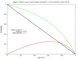
. as the prior, the probability of being uninfected post-test is 0.99757 vs 0.9932 pre-test. For all practical purposes, our knowledge has not improved.
 -axis). Note that graph 1 has an abbreviated
  , it provides near certainty of infection.
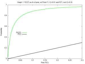
 and “sensitivity” refers to
  . See
. See  , de Rham Complex, review of some diff geom, Lie deriv and bracket, chain complexes, chain maps, homology, cochain complexes, cohomology, tie in to cat theory.
 : Used for a Principal bundle. Not really used here, but mentioned in passing.
 as a map from the de Rham complex to the singular cochain complex
 and
and  means
means and
and  : as
: as  -dimensional vector spaces over
  or as finite-basis modules over the smooth fns on M. The former is useful for abstract formulation while the latter is what we calculate with in DG. The transition between the two can be a source of confusion.
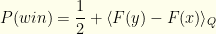
 regardless of whether we switch or not. But you weren’t asked to improve on the probability, just to maximize your expected payment. Consider the following 3 arguments:
 . If it is wrong to switch then the other envelope contains
  , but if it is right to switch it contains
  . There are even odds of either, so your expectation if you switch is
  . This is better than the
  . If it is wrong to switch then the envelope you chose contains
  , and if right to switch it contains
  . If you switch, you get
  . So it always is better NOT to switch!
  and
and  (though you don’t know which envelope contains which). You pick one, but there is equal probability of it being either
  . If you switch, the same holds true for the other envelope. So you still have an expected reward of
  . If we switch, then
  . If we keep the initial envelope then
  . Whether we switch or not, the expected value is
  or
or  . We must now draw an important distinction. It is correct that
  or
or  with equal probability. We defined
  . It determines which two numbers
  we are dealing with. We do not know
  with
with  . The envelopes thus contain
  for some integer
  (though we don’t know which envelope contains which value). For convenience, let’s work in terms of
  of the values involved (taking care to use
  for some
  (defined to be the lesser of the two). We open one, and see
  . If it is the upper then the pair is
  , otherwise the pair is
  . To claim that these have equal probabilities means that
  and
and  are equally probable. We made this assumption independent of the value of
  , so it would require that all pairs
  .
.
![{[M,N]}](https://s0.wp.com/latex.php?latex=%7B%5BM%2CN%5D%7D&bg=fefeeb&fg=000000&s=0&c=20201002) , which we supposedly know or assume apriori. We certainly can impose a uniform distribution on it. Each pair
, which we supposedly know or assume apriori. We certainly can impose a uniform distribution on it. Each pair  with
with ![{n\in [M,N-1]}](https://s0.wp.com/latex.php?latex=%7Bn%5Cin+%5BM%2CN-1%5D%7D&bg=fefeeb&fg=000000&s=0&c=20201002) . But now we’ve introduced additional information (in the form of
. But now we’ve introduced additional information (in the form of  and
and  ). For any
  and
and  . If we know
 ![\displaystyle \langle V_K \rangle= \sum_{n=-\infty}^\infty P(n) [P(m=n|n) 2^n + P(m=n+1|n) 2^{n+1}]](https://s0.wp.com/latex.php?latex=%5Cdisplaystyle+%5Clangle+V_K+%5Crangle%3D+%5Csum_%7Bn%3D-%5Cinfty%7D%5E%5Cinfty+P%28n%29+%5BP%28m%3Dn%7Cn%29+2%5En+%2B+P%28m%3Dn%2B1%7Cn%29+2%5E%7Bn%2B1%7D%5D&bg=fefeeb&fg=000000&s=0&c=20201002)
 for either of the two envelope orders. So we have
  . We immediately see that for this to be defined the probability distribution must drop faster than
 ![\displaystyle \langle V_S \rangle= \sum_{n=-\infty}^\infty P(n) [P(m=n|n) 2^{n+1} + P(m=n+1|n) 2^{n}]](https://s0.wp.com/latex.php?latex=%5Cdisplaystyle+%5Clangle+V_S+%5Crangle%3D+%5Csum_%7Bn%3D-%5Cinfty%7D%5E%5Cinfty+P%28n%29+%5BP%28m%3Dn%7Cn%29+2%5E%7Bn%2B1%7D+%2B+P%28m%3Dn%2B1%7Cn%29+2%5E%7Bn%7D%5D&bg=fefeeb&fg=000000&s=0&c=20201002)
 we get the same answer.
![\displaystyle \langle V_S \rangle= \sum_m P(m) [P(n=m|m) 2^{m+1} + P(n=m-1|m) 2^{m-1}]](https://s0.wp.com/latex.php?latex=%5Cdisplaystyle+%5Clangle+V_S+%5Crangle%3D+%5Csum_m+P%28m%29+%5BP%28n%3Dm%7Cm%29+2%5E%7Bm%2B1%7D+%2B+P%28n%3Dm-1%7Cm%29+2%5E%7Bm-1%7D%5D&bg=fefeeb&fg=000000&s=0&c=20201002)
 and
and  . We know that
  . Plugging these in, we get
![\displaystyle \langle V_S \rangle= \sum_m [0.5 P(n=m) 2^{m+1} + 0.5 P(n=m-1) 2^{m-1}]](https://s0.wp.com/latex.php?latex=%5Cdisplaystyle+%5Clangle+V_S+%5Crangle%3D+%5Csum_m+%5B0.5+P%28n%3Dm%29+2%5E%7Bm%2B1%7D+%2B+0.5+P%28n%3Dm-1%29+2%5E%7Bm-1%7D%5D&bg=fefeeb&fg=000000&s=0&c=20201002)
 . We can rewrite the index on the 2nd sum to get
  , which gives us
  , the exact same expression as before!
 exactly offsets the average gain from switching in all other cases. We do no better by switching than by keeping.
 or
or  but not both). To meaningfully analyze the problem we require a slightly stronger assumption, though: specifically that the set from which they be drawn (without repetition) possesses a strict linear ordering. However, it need not even possess any algebraic structure or a metric. Since we are not concerned with expectation values, no such additional structure is necessary.
 (i.e.
(i.e.  for all real
  stick with the initial choice, otherwise switch. We’ll refer to
  because the probability that
  has measure
  and safely can be ignored.
 glance, this seems pointless. It feels like all we’ve done is introduce a lot of cruft which will have no effect. We can go stand in a corner flipping a coin, play Baccarat at the local casino, cast the bones, or anything else we want, and none of that can change the probability that we’re equally likely to pick the lower envelope as the higher one initially — and thus equally likely to lose as to gain by switching. With no new information, there can be no improvement. Well, let’s hold that thought and do the calculation anyway. Just for fun.
 the values in the two envelopes in order. I.e.,
  by definition. In terms of
  and
and  . We’ll denote our contrived distribution
  and cdf
  .
.
 or
or  . So
. So  . There are no subtleties lurking here. We’ve assumed nothing about the underlying distribution over
  . Whatever
  and
and  and
and  . The latter forms the criterion by which we will keep
  is just notation for “the probability the sampled value is greater than

 and
and  since by assumption
  is monotonically increasing (we assumed its support is all of
  there is a greater probability that
  than
than  . We shouldn’t switch. A similar argument shows we should switch if
  .
.
 , of course. We’ll return to this shortly, but first let’s revisit the assumptions which make this work. We don’t need the envelopes to contain real numbers, but we do require the following of the values in the envelopes:
 is the true underlying distribution over
  since we are handed the envelopes to begin with. Perhaps the game is played many times with values drawn according to
  -distribution). Ultimately, such considerations just would divert us to the standard core philosophical questions of probability theory. Suffice to say that there exists some
  unless
  . We don’t employ a factor of
 ![\displaystyle \begin{array}{rcl} P(win)= \int_{x<y} dx dy Q(x,y)[p(z=x|(x,y))p(x<d) \\ + p(z=y|(x,y))p(d<y)] \end{array}](https://s0.wp.com/latex.php?latex=%5Cdisplaystyle++%5Cbegin%7Barray%7D%7Brcl%7D++P%28win%29%3D+%5Cint_%7Bx%3Cy%7D+dx+dy+Q%28x%2Cy%29%5Bp%28z%3Dx%7C%28x%2Cy%29%29p%28x%3Cd%29+%5C%5C+%2B+p%28z%3Dy%7C%28x%2Cy%29%29p%28d%3Cy%29%5D+%5Cend%7Barray%7D+&bg=fefeeb&fg=000000&s=0&c=20201002)
 since those are the immutable 50-50 envelope ordering probabilities. After a little rearrangement, we get:
 over the joint distribution
  . However, we cannot directly use
  because we defined
  and we don’t know whether
  or
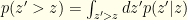
or  . Let’s start by computing the probability of
  (being the observed and unobserved values).

 we integrate this.
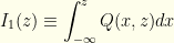
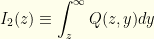
  . This is a good point to introduce two quantities which will be quite useful going forward.
![\displaystyle p(z)= \frac{1}{2}[I_1(z)+I_2(z)]](https://s0.wp.com/latex.php?latex=%5Cdisplaystyle+p%28z%29%3D+%5Cfrac%7B1%7D%7B2%7D%5BI_1%28z%29%2BI_2%28z%29%5D&bg=fefeeb&fg=000000&s=0&c=20201002)
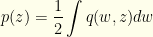
 . This gives us:
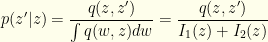
 . It is easy to see that:

 , we can figure that out.
  and
and  is the symmetrized version.
 ![{\int q(w,z)dw= \int dw [Q(w,z)+Q(z,w)]= (P_2(z/2)+P_2(2z))}](https://s0.wp.com/latex.php?latex=%7B%5Cint+q%28w%2Cz%29dw%3D+%5Cint+dw+%5BQ%28w%2Cz%29%2BQ%28z%2Cw%29%5D%3D+%28P_2%28z%2F2%29%2BP_2%282z%29%29%7D&bg=fefeeb&fg=000000&s=0&c=20201002) . So
. So  . This is just what we’d expect — though we’re really dealing with discrete values and are being sloppy (which ends us up with a ratio of infinities from the
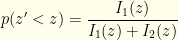
  . From a purely probability standpoint, we should switch if
  . If we reimpose the algebraic structure and try to compute expectations (as in the previous problem) we would get an expected value of
 ![{z[P_2(z/2)/2 + 2P(2z)]}](https://s0.wp.com/latex.php?latex=%7Bz%5BP_2%28z%2F2%29%2F2+%2B+2P%282z%29%5D%7D&bg=fefeeb&fg=000000&s=0&c=20201002) from switching . Whether this is less than or greater than
from switching . Whether this is less than or greater than  .
.
 directly. To optimize our probability of winning, we observe
  . If there is additional algebraic structure and expectations can be defined, then an analogous calculations give whatever switching criterion maximizes the relevant expectation value.
![\displaystyle \begin{array}{rcl} P'(win)= \int dz \frac{[\theta(I_1(z)-I_2(z)) I_1(z) + \theta(I_2(z)-I_1(z))I_2(z)]}{I_1(z)+I_2(z)} \\ = \int dz \frac{\max(I_1(z),I_2(z))}{(I_1(z)+I_2(z)} \end{array}](https://s0.wp.com/latex.php?latex=%5Cdisplaystyle++%5Cbegin%7Barray%7D%7Brcl%7D++P%27%28win%29%3D+%5Cint+dz+%5Cfrac%7B%5B%5Ctheta%28I_1%28z%29-I_2%28z%29%29+I_1%28z%29+%2B+%5Ctheta%28I_2%28z%29-I_1%28z%29%29I_2%28z%29%5D%7D%7BI_1%28z%29%2BI_2%28z%29%7D+%5C%5C+%3D+%5Cint+dz+%5Cfrac%7B%5Cmax%28I_1%28z%29%2CI_2%28z%29%29%7D%7B%28I_1%28z%29%2BI_2%28z%29%7D+%5Cend%7Barray%7D+&bg=fefeeb&fg=000000&s=0&c=20201002)

 and
and  are monotonic (one increasing, the other decreasing), we have a cutoff value
  (defined by
  ) below which we should switch and above which we should not.
 into our current notation, but it’s easier to compute directly. For given
  . Based on our algorithm, we will do so with probability
  . The probability of not needing to switch is
  and we do so with probability
  . I.e., our probability of success for given
 where
where  and
and  . The optimal solutions lie at one end or the other. So it obviously is best to have
  when
when  and
and  when
when  . This would be discontinuous, but we could come up with a smoothed step function (ex. a logistic function) which is differentiable but arbitrarily sharp. The gist is that we want all the probability in
  . Integrating over
  . I.e., We end up with
  as our probability of success. If we had used
  for our
  instead. Neither is optimal in general.
![{p(z)=\frac{1}{2}[I_1(z)+I_2(z)]}](https://s0.wp.com/latex.php?latex=%7Bp%28z%29%3D%5Cfrac%7B1%7D%7B2%7D%5BI_1%28z%29%2BI_2%28z%29%5D%7D&bg=fefeeb&fg=000000&s=0&c=20201002) . Given that
. Given that  given by
  ) is
) is
![\displaystyle H(z'>z|z)= \frac{-I_1(z)\ln I(z) - I_2(z)\ln I_2(z) + (I_1(z)+I_2(z))\ln [I_1(z)+I_2(z)]}{I_1(z)+I_2(z)}](https://s0.wp.com/latex.php?latex=%5Cdisplaystyle+H%28z%27%3Ez%7Cz%29%3D+%5Cfrac%7B-I_1%28z%29%5Cln+I%28z%29+-+I_2%28z%29%5Cln+I_2%28z%29+%2B+%28I_1%28z%29%2BI_2%28z%29%29%5Cln+%5BI_1%28z%29%2BI_2%28z%29%5D%7D%7BI_1%28z%29%2BI_2%28z%29%7D&bg=fefeeb&fg=000000&s=0&c=20201002)
 . This yields a conditional entropy:

 the probability based on the true distribution and keep
  and
and ![\displaystyle D(Q || P, z)= \frac{-I_2(z)\ln [(I_1(z)+I_2(z))(1-F(z))/I_2(z)] - I_1(z)\ln [(I_1(z)+I_2(z))F(z)/I_1(z)]}{I_1(z)+I_2(z)}](https://s0.wp.com/latex.php?latex=%5Cdisplaystyle+D%28Q+%7C%7C+P%2C+z%29%3D+%5Cfrac%7B-I_2%28z%29%5Cln+%5B%28I_1%28z%29%2BI_2%28z%29%29%281-F%28z%29%29%2FI_2%28z%29%5D+-+I_1%28z%29%5Cln+%5B%28I_1%28z%29%2BI_2%28z%29%29F%28z%29%2FI_1%28z%29%5D%7D%7BI_1%28z%29%2BI_2%28z%29%7D&bg=fefeeb&fg=000000&s=0&c=20201002)
![\displaystyle \begin{array}{rcl} \langle D(Q || P) \rangle= \frac{1}{2}\int dz [-(I_1(z)+I_2(z))\ln [I_1(z)+I_2(z)] - I_2(z)\ln (1-F(z)) \\ -I_1(z)\ln F(z) + I_1(z)\ln I_1(z) + I_2(z)\ln I_2(z)] \end{array}](https://s0.wp.com/latex.php?latex=%5Cdisplaystyle++%5Cbegin%7Barray%7D%7Brcl%7D++%5Clangle+D%28Q+%7C%7C+P%29+%5Crangle%3D+%5Cfrac%7B1%7D%7B2%7D%5Cint+dz+%5B-%28I_1%28z%29%2BI_2%28z%29%29%5Cln+%5BI_1%28z%29%2BI_2%28z%29%5D+-+I_2%28z%29%5Cln+%281-F%28z%29%29+%5C%5C+-I_1%28z%29%5Cln+F%28z%29+%2B+I_1%28z%29%5Cln+I_1%28z%29+%2B+I_2%28z%29%5Cln+I_2%28z%29%5D+%5Cend%7Barray%7D+&bg=fefeeb&fg=000000&s=0&c=20201002)
 , the entropy of our actual distribution over
  , the mean Bernoulli entropy of the actual distribution. In these terms, we have:

 where
where  is the always-keep strategy,
  is the always-switch strategy, and
  is the probability of employing the always-keep strategy. A player would flip a biased-coin with Bernoulli probability
  and choose one of the two-strategies based on it. That has nothing to do with the measure-theory approach we’re taking here. In particular, a mixes strategy makes no use of the observed value