bayesian inference | A Place of Sand

I’ve recently been reviewing Bayesian networks with an eye to learning STAN. One question which occurred to me is the following. Suppose we are interested in the probability distribution $P(\mu)$ over parameters $\mu\in X$ (with state space $X$ ). We acquire some data $D$ , and wish to use it to infer $P(\mu)$ . Note that $D$ refers to the specific realized data, not the event space from which it is drawn.

Let’s assume that (1) we have a prior $P(\mu)$ , (2) the likelihood $P(D|\mu)$ is easy to compute or sample, and (3) the normalization 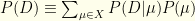$P(D)\equiv \sum_{\mu\in X} P(D|\mu)P(\mu)$ is not expensive to compute or adequately approximate.

The usual Bayesian approach involves updating the prior to a posterior via Bayes’ thm: $P(\mu|D)= \frac{P(D|\mu)P(\mu)}{P(D)}$ . However, there also is another view we may take. We need not restrict ourselves to a single Bayesian update. It is perfectly reasonable to ask whether multiple updates using the same $D$ would yield a more useful result.

Such a tactic is not as ridiculous or unjustified as it first seems. In many cases, the Bayesian posterior is highly sensitive to a somewhat arbitrary choice of prior $P(\mu)$ . The latter frequently is dictated by practical considerations rather than arising naturally from the problem at hand. For example, we often use the likelihood function’s conjugate prior to ensure that the posterior will be of the same family. Even in this case, the posterior depends heavily on the precise choice of $P(\mu)$ .

Though we must be careful interpreting the results, there very well may be applications in which an iterated approach is preferable. For example, it is conceivable that multiple iterations could dilute the dependence on $P(\mu)$ , emphasizing the role of $D$ instead. We can seek inspiration in the stationary distributions of Markov chains, where the choice of initial distribution becomes irrelevant. As a friend of mine likes to say before demolishing me at chess: let’s see where this takes us. Spoiler: infinite iteration “takes us” to maximum-likelihood selection.

An iterated approach does not violate any laws of probability. Bayes’ thm is based on the defining property $P(\mu,D)= P(D|\mu)P(\mu)= P(\mu|D)P(D)$ . Our method is conceptually equivalent to performing successive experiments which happen to produce the same data $D$ each time, reinforcing our certainty around it. Although its genesis is different, the calculation is the same. I.e., any inconsistency or inapplicability must arise through interpretation rather than calculation. The results of an iterated calculation may be inappropriate for certain purposes (such as estimating error bars, etc), but could prove useful for others.

In fact, one could argue there only are two legitimate approaches when presented with a one-time data set $D$ . We could apply it once or an infinite number of times. Anything else would amount to an arbitrary choice of the number of iterations.

It is easy to analyze the infinite iteration process. For simplicity, we’ll consider the case of a discrete, finite state space $X$ . $D$ is a fixed set of data values for our problem, so we are not concerned with the space or distribution from which it is drawn. $P(D)$ is a derived normalization factor, nothing more.

Let’s introduce some notation:

– Let $n\equiv |X|$ , and denote the elements of $X$ by $\mu_1\dots \mu_n$ .
– We could use $n$ -vectors to denote probability or conditional probability distributions over $X$ (with the $i^{th}$ component the probability of $\mu_i$ ), but it turns out to be simpler to use diagonal $n\times n$ matrices.
– $P(\mu)$ is an $n$ -vector, which we’ll write as a diagonal $n\times n$ matrix $v$ with $v_{ii}\equiv P(\mu_i)$ .
– We’ll denote by $D^k$ the data set $D$ repeated $k$ times. I.e., the equivalent of having performed an experiment $k$ times and obtained $D$ each time.
– $P(\mu|D)$ is an $n$ -vector, which we’ll write as a diagonal $n\times n$ matrix $v'$ with $v'_{ii}\equiv P(\mu_i|D)$ ).
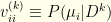– Where multiple updates are involved, we denote the final posterior $P(\mu|D^k)$ via an $n\times n$ diagonal matrix $v^{(k)}$ , with $v^{(k)}_{ii}\equiv P(\mu_i|D^k)$ . Note that $v'= v^{(1)}$ and $v= v^{(0)}$ .
– $P(D|\mu)$ as an $n$ -vector of probabilities as well, but we’ll also treat it as a diagonal $n\times n$ matrix $M$ with $M_{ii}\equiv P(D|\mu_i)$ .
– $P(D)=\sum_{i=1}^n P(D|\mu_i)P(\mu_i)$ is a scalar. In our notation, $P(D)= \text{tr}~ M v$ .

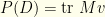A single Bayesian update takes the form $v'= M v/(\text{tr}~ M v)$ . What happens if we repeat this? A second iteration substitutes $v'$ for $v$ , and we get $v^{(2)}= M v'/(\text{tr}~ M v')$ . This is homogeneous of degree $0$ in $v'$ , so the $(\text{tr}~ M v)$ normalization factor in $v'$ disappears. We thus have 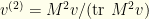$v^{(2)}= M^2 v /(\text{tr}~ M^2 v)$ . The same reasoning extends to $v^{(k)}= M^k v/(\text{tr}~ M^k v)$ .

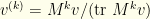It now is easy to see what is happening. Suppose $n=2$ , and let $M_{11}>M_{22}$ . Our expression for $P(\mu_1|D)$ after $k$ iterations is $v^{(k)}_1= \frac{M^k_{11} v_{11}}{M^k_{11} v_{11} + M^k_{22} v_{22}}$ .

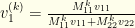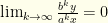This has the form $\frac{a^k x}{a^k x + b^k y}$ , which can be written $1/(1+\frac{b^k y}{a^k x})$ . We know that $b<a$ , so as long as $x\ne 0$ we have $\lim_{k\rightarrow\infty} \frac{b^k y}{a^k x}= 0$ . Specifically, for $\epsilon>0$ we have $\frac{b^k y}{a^k x}<\epsilon$ for $k>\frac{\ln\epsilon + \ln \frac{x}{y}}{\ln \frac{b}{a}}$ . Note that the denominator is negative since $a>b$ and the numerator is negative for small enough $\epsilon$ .

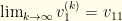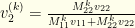We therefore have shown that (in this simple case), $\lim_{k\rightarrow\infty} v^{(k)}_1= v_{11}$ . If we perform the same analysis for $v^{(k)}_2$ , we get $v^{(k)}_2= \frac{M^k_{22} v_{22}}{M^k_{11} v_{11} + M^k_{22} v_{22}}$ , which corresponds to $1/(1+\frac{a^k x}{b^k y})$ . The denominator diverges for large enough $k$ , and the limit is $0$ . We therefore see that $\lim_{k\rightarrow\infty} v^{(k)}_2= 0$ .

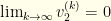This trivially extends to $n>2$ . As $k\rightarrow\infty$ , all but the dominant $M_{ii}$ are exponentially suppressed. The net effect of infinite iteration is to pick out the maximum likelihood value. I.e., we select the $\mu_i$ corresponding to the maximum $M_{ii}$ . All posterior probability is concentrated in that. 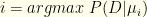Put another way, the limit of iterated posteriors is $P(\mu_i|D^\infty)= 1$ for $i=argmax~P(D|\mu_i)$ and $0$ for all others.

What if the maximum $M_{ii}$ is degenerate? Let’s again consider the simple $n=2$ case, but now with $M_{11}= M_{22}>0$ . It is easy to see what happens in this case. $a/b=1$ , so $v^{(k)}_1= \frac{v_{11}}{v_{11}+v_{22}}$ and $v^{(k)}_2= \frac{v_{22}}{v_{11}+v_{22}}$ . Note that $v_{11}+v_{22}=1$ here, but we stated the denominator explicitly to facilitate visualization of the extension to $n>2$ .

This extension is straightforward. We pick out the maximum likelihood values $\mu_i$ , and they are assigned their prior probabilities, renormalized. Suppose there are $m\le n$ degenerate maximum $M_{ii}$ ‘s, with indices $i_1\dots i_m$ (each $i_j\in 1\dots n$ ). The limit of iterated posteriors $P(\mu_{i_j}|D^\infty)= \frac{P(\mu_i)}{\sum_{j=1}^m P(\mu_{i_j})}$ . This reduces to our previous result when $m=1$ .

Note that we must ensure $v_i\ne 0$ for the maximum likelihood $\mu_i$ ‘s. I.e., we cannot have a $0$ prior for any of the maximum likelihood values. If we wish to exclude $\mu_i$ ‘s from consideration, we should do so before the calculation, thus eliminating the corresponding $P(D|\mu_i)$ ‘s from contention for the maximum likelihood.

Expanding $|X|$ to a countable set poses no problem. In the continuous case, we must work with intervals (or measurable sets) rather than point values. For any $\epsilon>0$ and any set of nonzero measure containing all the maximum likelihood values, there will be some $k$ that concentrates all but $\epsilon$ of the posterior probability in that set.

Note that $k$ depends on the choice of measurable set, and care must be taken when considering limits of such sets. For example, let $p\equiv \max_{\mu} P(D|\mu)$ be the maximum likelihood probability. If we consider an interval $I\equiv (p-\delta/2,p+\delta/2)$ as our maximum likelihood set, then the maximum likelihood “value” is the (measurable) set $V\equiv P(D|\mu)^{-1}(I)$ . For any $\epsilon$ , we have a $k$ as discussed above, such that $P(\mu\notin V|D^j)<\epsilon$ for $j>k$ . However, for a fixed $\epsilon$ , that $k$ will vary with $\delta$ . Put another way, we cannot simply assume uniform convergence.

We can view infinite iteration as a modification of the prior. Specifically, it is tantamount to pruning the prior of all non-maximum-likelihood values and renormalizing it accordingly. The posterior then is equal to the prior under subsequent single- $D$ steps (i.e. it is a fixed point distribution). Alternatively, we can view the whole operation as a single $D^\infty$ update. In that case, we keep the original prior and view the posterior as the aforementioned pruned version of the prior.

There are two takeaways here:

1. The infinite iteration approach simply amounts to maximum-likelihood selection. It selects the maximum likelihood value(s) from the known $P(D|\mu)$ and maintains their relative prior probabilities, suitably renormalized. Equivalently, it prunes all the non-maximum-likelihood values.
2. The resulting posterior still depends on the choice of prior unless the maximum likelihood value is unique, in which case that value has probability $1$ .

Unlike stationary distributions of Markov chains, the result is not guaranteed to be independent of our arbitrary initial choice — in this case, the prior $P(\mu)$ . Though true independence only is achieved when there is a unique maximum likelihood value, the dependence is reduced significantly even when there is not. The posterior depends only on those prior values corresponding to maximum likelihood $\mu$ ‘s. All others are irrelevant. The maximum likelihood values typically form a tiny subset of $\mu$ ‘s, thus eliminating most dependence on the prior. Note that such degeneracy (as well as the values themselves) is solely determined by the likelihood function.