Tag Archives: mathy

Semidirect Products, Group Extensions, Split Exact Sequences, and all that

July 8, 2023 K.M. Halpern

UPDATED SUBSTANTIALLY 7/6/2023
[Original Version Posted 1/22/2019]

PDF Notes: Semidirect Products, Group Extensions, Split Exact Sequences, and all that

If you suffer physics-brain and don’t know anything about semidirect products or group extensions, but get the sense direct products just aren’t cutting it — these are the notes for you.

Update: On reexamination, my original post on the subject was too brief and simplistic. Among other things, it neglected to explicitly construct the multiplication on a group extension. In the process of doing so, I identified numerous other shortcomings and omissions. As a result, I’ve replaced it with a far more thorough discussion. Unfortunately, at 50 pages it has expanded beyond the point where the primitive wordpress support for latex suffices. The notes now are provided as a pdf (linked at the top and bottom of this post). This has the added benefit of allowing me to the color-code proofs and comments and examples, allowing easier reading of the key elements.

The purpose of this post is to cure one aspect of physics-brain. In a typical physics education, we learn a sloppy version of linear algebra, basic group theory, and (certain) differential equations many times — and little else math-related. As a result, we develop numerous bad habits and suffer from a complete ignorance of certain important areas of mathematics. If two groups are being combined, it’s via a direct product. After all, what else is there? Unfortunately, this only works until it doesn’t — which is pretty much anywhere it matters. For example, even O(3,1) is not a direct product of the 2 copies of Z2 and SO+(3,1). You’ve probably heard of O(3,1). It matters.

Many of the things we naively assume would be direct products actually are semidirect products or general group extensions, and the result can be a lot of confusion when things don’t work as expected. Besides the construction of basic physical groups such as the Poincare group, this also arises in the study of quantum mechanics. Part of the reason we can pretend to work in Hilbert space when the actual state space is a projective Hilbert space is that the projective representations of a group lift to unitary representations of a different group. The latter is a particular group extension (in fact, a central extension) of the original group.

Ignorance of semidirect products and group extensions is quite understandable in a physicist, but also easily cured. These notes are an attempt to do so based on my experience trying to cure myself. They are self-contained, and the only prerequisite is a little group theory. Though I allude to topology in a couple of places, no knowledge of it is necessary.

These notes cover the following:

Normal subgroups and quotient groups, the isomorphism thms, various other group-related concepts, and inner/outer automorphisms.
Exact sequences, short-exact-sequences (SES’s), splitting of SES’s, central extensions, and the isomorphism classes of SES’s (as well as how they interact with splitting).
Introduction to the hierarchy of direct products, semidirect products, and group extensions. We take 3 views of each: (1) an external view in which we build a new group from two distinct groups, (2) an internal view in which we consider the relationship between an existing group and its subgroups, and (3) an SES-view in which we frame things in terms of short exact sequences. Because the external-view is conceptually the most challenging, we give a preview of its regimen.
The direct product in all 3 views.
Semidirect products in all 3 views.
General group extensions in all 3 views.
A brief comparison of direct products, semidirect products, and group extensions in all 3 views.
An addendum in which we explicitly construct the multiplication on a group extension in gory detail.

A few caveats. There are lots of detailed proofs in the notes. There also probably are typos and possibly errors. I hope to correct and clarify as needed, so please report these to me if you encounter any. The notes were written in passes and phases. There is a lot of intentional replication of effort in the proofs (where it serves the purpose of clarity), but also probably some unintentional replication (for example, if I consolidated some results in a proposition in one place, but fail to use those results in another). Nonetheless, I believe they should be quite informative and are on balance both correct and quite comprehensible. In particular, I tried to avoid “simplifying” things in subsequent passes as my understanding improved (though I certainly did correct things as needed). The danger in doing so is that I would lose sight of the things which confused me when first encountering the concepts — and one purpose of these notes is to address such sources of confusion. After enough passes and simplifications, the entire piece would end up a one page terse Bourbaki-like statement, along with a vague hint at the possibility of an idea of a proof-outline — which anyone worth their salt is expected to easily be able to expand into a 40-page proof. In math, the best way to learn a subject is to already know it. In physics, we take a gentler approach.

There are a couple of key omission — neither mission-central — which I hope to address in future posts. These concern (1) the relationship between semidirect products/group extensions and fiber bundles/principal bundles and (2) a detailed discussion of group cohomology and the classification of group extensions.

PDF Notes: Semidirect Products, Group Extensions, Split Exact Sequences, and all that

Notes

What happens when you iterate Bayesian Inference with the same data set?

November 28, 2021 K.M. Halpern Leave a comment

I’ve recently been reviewing Bayesian networks with an eye to learning STAN. One question which occurred to me is the following. Suppose we are interested in the probability distribution $P(\mu)$ over parameters $\mu\in X$ (with state space $X$ ). We acquire some data $D$ , and wish to use it to infer $P(\mu)$ . Note that $D$ refers to the specific realized data, not the event space from which it is drawn.

Let’s assume that (1) we have a prior $P(\mu)$ , (2) the likelihood $P(D|\mu)$ is easy to compute or sample, and (3) the normalization $P(D)\equiv \sum_{\mu\in X} P(D|\mu)P(\mu)$ is not expensive to compute or adequately approximate.

The usual Bayesian approach involves updating the prior to a posterior via Bayes’ thm: $P(\mu|D)= \frac{P(D|\mu)P(\mu)}{P(D)}$ . However, there also is another view we may take. We need not restrict ourselves to a single Bayesian update. It is perfectly reasonable to ask whether multiple updates using the same $D$ would yield a more useful result.

Such a tactic is not as ridiculous or unjustified as it first seems. In many cases, the Bayesian posterior is highly sensitive to a somewhat arbitrary choice of prior $P(\mu)$ . The latter frequently is dictated by practical considerations rather than arising naturally from the problem at hand. For example, we often use the likelihood function’s conjugate prior to ensure that the posterior will be of the same family. Even in this case, the posterior depends heavily on the precise choice of $P(\mu)$ .

Though we must be careful interpreting the results, there very well may be applications in which an iterated approach is preferable. For example, it is conceivable that multiple iterations could dilute the dependence on $P(\mu)$ , emphasizing the role of $D$ instead. We can seek inspiration in the stationary distributions of Markov chains, where the choice of initial distribution becomes irrelevant. As a friend of mine likes to say before demolishing me at chess: let’s see where this takes us. Spoiler: infinite iteration “takes us” to maximum-likelihood selection.

An iterated approach does not violate any laws of probability. Bayes’ thm is based on the defining property $P(\mu,D)= P(D|\mu)P(\mu)= P(\mu|D)P(D)$ . Our method is conceptually equivalent to performing successive experiments which happen to produce the same data $D$ each time, reinforcing our certainty around it. Although its genesis is different, the calculation is the same. I.e., any inconsistency or inapplicability must arise through interpretation rather than calculation. The results of an iterated calculation may be inappropriate for certain purposes (such as estimating error bars, etc), but could prove useful for others.

In fact, one could argue there only are two legitimate approaches when presented with a one-time data set $D$ . We could apply it once or an infinite number of times. Anything else would amount to an arbitrary choice of the number of iterations.

It is easy to analyze the infinite iteration process. For simplicity, we’ll consider the case of a discrete, finite state space $X$ . $D$ is a fixed set of data values for our problem, so we are not concerned with the space or distribution from which it is drawn. $P(D)$ is a derived normalization factor, nothing more.

Let’s introduce some notation:

– Let $n\equiv |X|$ , and denote the elements of $X$ by $\mu_1\dots \mu_n$ .
– We could use $n$ -vectors to denote probability or conditional probability distributions over $X$ (with the $i^{th}$ component the probability of $\mu_i$ ), but it turns out to be simpler to use diagonal $n\times n$ matrices.
– $P(\mu)$ is an $n$ -vector, which we’ll write as a diagonal $n\times n$ matrix $v$ with $v_{ii}\equiv P(\mu_i)$ .
– We’ll denote by $D^k$ the data set $D$ repeated $k$ times. I.e., the equivalent of having performed an experiment $k$ times and obtained $D$ each time.
– $P(\mu|D)$ is an $n$ -vector, which we’ll write as a diagonal $n\times n$ matrix $v'$ with $v'_{ii}\equiv P(\mu_i|D)$ ).
– Where multiple updates are involved, we denote the final posterior $P(\mu|D^k)$ via an $n\times n$ diagonal matrix $v^{(k)}$ , with $v^{(k)}_{ii}\equiv P(\mu_i|D^k)$ . Note that $v'= v^{(1)}$ and $v= v^{(0)}$ .
– $P(D|\mu)$ as an $n$ -vector of probabilities as well, but we’ll also treat it as a diagonal $n\times n$ matrix $M$ with $M_{ii}\equiv P(D|\mu_i)$ .
– $P(D)=\sum_{i=1}^n P(D|\mu_i)P(\mu_i)$ is a scalar. In our notation, $P(D)= \text{tr}~ M v$ .

A single Bayesian update takes the form $v'= M v/(\text{tr}~ M v)$ . What happens if we repeat this? A second iteration substitutes $v'$ for $v$ , and we get $v^{(2)}= M v'/(\text{tr}~ M v')$ . This is homogeneous of degree $0$ in $v'$ , so the $(\text{tr}~ M v)$ normalization factor in $v'$ disappears. We thus have $v^{(2)}= M^2 v /(\text{tr}~ M^2 v)$ . The same reasoning extends to $v^{(k)}= M^k v/(\text{tr}~ M^k v)$ .

It now is easy to see what is happening. Suppose $n=2$ , and let $M_{11}>M_{22}$ . Our expression for $P(\mu_1|D)$ after $k$ iterations is $v^{(k)}_1= \frac{M^k_{11} v_{11}}{M^k_{11} v_{11} + M^k_{22} v_{22}}$ .

This has the form $\frac{a^k x}{a^k x + b^k y}$ , which can be written $1/(1+\frac{b^k y}{a^k x})$ . We know that $b<a$ , so as long as $x\ne 0$ we have $\lim_{k\rightarrow\infty} \frac{b^k y}{a^k x}= 0$ . Specifically, for $\epsilon>0$ we have $\frac{b^k y}{a^k x}<\epsilon$ for $k>\frac{\ln\epsilon + \ln \frac{x}{y}}{\ln \frac{b}{a}}$ . Note that the denominator is negative since $a>b$ and the numerator is negative for small enough $\epsilon$ .

We therefore have shown that (in this simple case), $\lim_{k\rightarrow\infty} v^{(k)}_1= v_{11}$ . If we perform the same analysis for $v^{(k)}_2$ , we get $v^{(k)}_2= \frac{M^k_{22} v_{22}}{M^k_{11} v_{11} + M^k_{22} v_{22}}$ , which corresponds to $1/(1+\frac{a^k x}{b^k y})$ . The denominator diverges for large enough $k$ , and the limit is $0$ . We therefore see that $\lim_{k\rightarrow\infty} v^{(k)}_2= 0$ .

This trivially extends to $n>2$ . As $k\rightarrow\infty$ , all but the dominant $M_{ii}$ are exponentially suppressed. The net effect of infinite iteration is to pick out the maximum likelihood value. I.e., we select the $\mu_i$ corresponding to the maximum $M_{ii}$ . All posterior probability is concentrated in that. Put another way, the limit of iterated posteriors is $P(\mu_i|D^\infty)= 1$ for $i=argmax~P(D|\mu_i)$ and $0$ for all others.

What if the maximum $M_{ii}$ is degenerate? Let’s again consider the simple $n=2$ case, but now with $M_{11}= M_{22}>0$ . It is easy to see what happens in this case. $a/b=1$ , so $v^{(k)}_1= \frac{v_{11}}{v_{11}+v_{22}}$ and $v^{(k)}_2= \frac{v_{22}}{v_{11}+v_{22}}$ . Note that $v_{11}+v_{22}=1$ here, but we stated the denominator explicitly to facilitate visualization of the extension to $n>2$ .

This extension is straightforward. We pick out the maximum likelihood values $\mu_i$ , and they are assigned their prior probabilities, renormalized. Suppose there are $m\le n$ degenerate maximum $M_{ii}$ ‘s, with indices $i_1\dots i_m$ (each $i_j\in 1\dots n$ ). The limit of iterated posteriors $P(\mu_{i_j}|D^\infty)= \frac{P(\mu_i)}{\sum_{j=1}^m P(\mu_{i_j})}$ . This reduces to our previous result when $m=1$ .

Note that we must ensure $v_i\ne 0$ for the maximum likelihood $\mu_i$ ‘s. I.e., we cannot have a $0$ prior for any of the maximum likelihood values. If we wish to exclude $\mu_i$ ‘s from consideration, we should do so before the calculation, thus eliminating the corresponding $P(D|\mu_i)$ ‘s from contention for the maximum likelihood.

Expanding $|X|$ to a countable set poses no problem. In the continuous case, we must work with intervals (or measurable sets) rather than point values. For any $\epsilon>0$ and any set of nonzero measure containing all the maximum likelihood values, there will be some $k$ that concentrates all but $\epsilon$ of the posterior probability in that set.

Note that $k$ depends on the choice of measurable set, and care must be taken when considering limits of such sets. For example, let $p\equiv \max_{\mu} P(D|\mu)$ be the maximum likelihood probability. If we consider an interval $I\equiv (p-\delta/2,p+\delta/2)$ as our maximum likelihood set, then the maximum likelihood “value” is the (measurable) set $V\equiv P(D|\mu)^{-1}(I)$ . For any $\epsilon$ , we have a $k$ as discussed above, such that $P(\mu\notin V|D^j)<\epsilon$ for $j>k$ . However, for a fixed $\epsilon$ , that $k$ will vary with $\delta$ . Put another way, we cannot simply assume uniform convergence.

We can view infinite iteration as a modification of the prior. Specifically, it is tantamount to pruning the prior of all non-maximum-likelihood values and renormalizing it accordingly. The posterior then is equal to the prior under subsequent single- $D$ steps (i.e. it is a fixed point distribution). Alternatively, we can view the whole operation as a single $D^\infty$ update. In that case, we keep the original prior and view the posterior as the aforementioned pruned version of the prior.

There are two takeaways here:

1. The infinite iteration approach simply amounts to maximum-likelihood selection. It selects the maximum likelihood value(s) from the known $P(D|\mu)$ and maintains their relative prior probabilities, suitably renormalized. Equivalently, it prunes all the non-maximum-likelihood values.
2. The resulting posterior still depends on the choice of prior unless the maximum likelihood value is unique, in which case that value has probability $1$ .

Unlike stationary distributions of Markov chains, the result is not guaranteed to be independent of our arbitrary initial choice — in this case, the prior $P(\mu)$ . Though true independence only is achieved when there is a unique maximum likelihood value, the dependence is reduced significantly even when there is not. The posterior depends only on those prior values corresponding to maximum likelihood $\mu$ ‘s. All others are irrelevant. The maximum likelihood values typically form a tiny subset of $\mu$ ‘s, thus eliminating most dependence on the prior. Note that such degeneracy (as well as the values themselves) is solely determined by the likelihood function.

Research

CCSearch State Space Algo

October 15, 2019 K.M. Halpern

While toying with automated Fantasy Sports trading systems, I ended up designing a rapid state search algorithm that was suitable for a variety of constrained knapsack-like problems.

A reference implementation can be found on github: https://github.com/kensmosis/ccsearch.

Below is a discussion of the algorithm itself. For more details, see the source code in the github repo. Also, please let me know if you come across any bugs! This is a quick and dirty implementation.

Here is a description of the algorithm:

— Constrained Collection Search Algorithm —

Here, we discuss a very efficient state-space search algorithm which originated with a Fantasy Sports project but is applicable to a broad range of applications. We dub it the Constrained Collection Search Algorithm for want of a better term. A C++ implementation, along with Python front-end is included as well.

In the Fantasy Sports context, our code solves the following problem: We’re given a tournament with a certain set of rules and requirements, a roster of players for that tournament (along with positions, salaries and other info supplied by the tournament’s host), and a user-provided performance measure for each player. We then search for those teams which satisfy all the constraints while maximizing team performance (based on the player performances provided). We allow a great deal of user customization and flexibility, and currently can accommodate (to our knowledge) all major tournaments on Draftkings and FanDuel. Through aggressive pruning, execution time is minimized.

As an example, on data gleaned from some past Fantasy Baseball tournaments, our relatively simple implementation managed to search a state space of size approximately ${10^{21}}$ unconstrained fantasy teams, ultimately evaluating under ${2}$ million plausible teams and executing in under ${4}$ seconds on a relatively modest desktop computer.

Although originating in a Fantasy Sport context, the CCSearch algorithm and code is quite general.

— Motivating Example —

We’ll begin with the motivating example, and then consider the more abstract case. We’ll also discuss some benchmarks and address certain performance considerations.

In Fantasy Baseball, we are asked to construct a fantasy “team” from real players. While the details vary by platform and tournament, such games share certain common elements:

A “roster”. This is a set of distinct players for the tournament.
A means of scoring performance of a fantasy team in the tournament. This is based on actual performance by real players in the corresponding games. Typically, each player is scored based on certain actions (perhaps specific to their position), and these player scores then are added to get the team score.
For each player in the roster, the following information (all provided by the tournament host except for the predicted fantasy-points, which generally is based on the user’s own model of player performance):

A “salary”, representing the cost of inclusion in our team.
A “position” representing their role in the game.
One or more categories they belong to (ex. pitcher vs non-pitcher, real team they play on).
A prediction of the fantasy-points the player is likely to score.

A number ${N}$ of players which constitute a fantasy team. A fantasy team must have precisely this number of players.

A salary cap. This is the maximum sum of player salaries we may “spend” in forming a fantasy team. Most, but not all, tournaments have one.

A set of positions, and the number of players in each. The players on our team must adhere to these. For example, we may have ${3}$ players from one position and ${2}$ from another and ${1}$ each from ${4}$ other positions. Sometimes there are “flex” positions, and we’ll discuss how to accommodate those as well. The total players in all the positions must sum to ${N}$ .

Various other constraints on team formation. These come in many forms and we’ll discuss them shortly. They keep us from having too many players from the same real-life team, etc.

To give a clearer flavor, let’s consider a simple example: Draftkings Fantasy Baseball. There are at least 7 Tournament types listed (the number and types change with time, so this list may be out of date). Here are some current game types. For each, there are rules for scoring the performance of players (depending on whether hitter or pitcher, and sometimes whether relief or starting pitcher — all of which info the tournament host provides):

Classic: ${N=10}$ players on a team, with specified positions P,P,C,1B,2B,3B,SS,OF,OF,OF. Salary cap is $50K. Constraints: (1) ${\le 5}$ hitters (non-P players) from a given real team, and (2) players from ${\ge 2}$ different real games must be present.
Tiers: ${N}$ may vary. A set of performance “tiers” is provided by the host, and we pick one player from each tier. There is no salary cap, and the constraint is that players from ${\ge 2}$ different real games must be present.
Showdown: ${N=6}$ players, with no position requirements. Salary cap is $50K. Constraints: (1) players from ${\ge 2}$ different real teams, and (2) ${\le 4}$ hitters from any one team.
Arcade: ${N=6}$ players, with 1 pitcher, 5 hitters. Salary cap is $50K. Constraints are: (1) ${\le 3}$ hitters (non-P players) from a given real team, and (2) players from ${\ge 2}$ different real games must be present.
Playoff Arcade: ${N=7}$ players, with 2 pitchers and 5 hitters. Salary cap is $50K. Constraints are: (1) ${\le 3}$ hitters (non-P players) from a given real team, and (2) players from ${\ge 2}$ different real games must be present.
Final Series (involves 2 games): ${N=8}$ players, with 2 pitchers and 6 hitters. $50K salary cap. Constraints are: (1) ${1}$ pitcher from each of the two games, (2) ${3}$ hitters from each of the the ${2}$ games, (3) can’t have the same player twice (even if they appear in both games), and (4) Must have hitters from both teams in each game.
Lowball: Same as Tiers, but the lowest score wins.

Although the constraints above may seem quite varied, we will see they fall into two easily-codified classes.

In the Classic tournament, we are handed a table prior to the competition. This contains a roster of available players. In theory there would be 270 (9 for each of the 30 teams), but not every team plays every day and there may be injuries so it can be fewer in practice. For each player we are given a field position (P,C,1B,2B,3B,SS,or OF), a Fantasy Salary, their real team, and which games they will play in that day. For our purposes, we’ll assume they play in a single game on a given day, though it’s easy to accommodate more than one.

Let us suppose that we have a model for predicting player performance, and are thus also provided with a mean and standard deviation performance. This performance is in terms of “points”, which is Draftkings’ scoring mechanism for the player. I.e., we have a prediction for the score which Draftkings will assign the player using their (publicly available) formula for that tournament and position. We won’t discuss this aspect of the process, and simply take the predictive model as given.

Our goal is to locate the fantasy teams which provide the highest combined predicted player scores while satisfying all the requirements (position, salary, constraints) for the tournament. We may wish to locate the top ${L}$ such teams (for some ${L}$ ) or all those teams within some performance distance of the best.

Note that we are not simply seeking a single, best solution. We may wish to bet on a set of 20 teams which diversify our risk as much as possible. Or we may wish to avoid certain teams in post-processing, for reasons unrelated to the constraints.

It is easy to see that in many cases the state space is enormous. We could attempt to treat this as a knapsack problem, but the desire for multiple solutions and the variety of constraints make it difficult to do so. As we will see, an aggressively pruned direct search can be quite efficient.

— The General Framework —

There are several good reasons to abstract this problem. First, it is the sensible mathematical thing to do. It also offers a convenient separation from a coding standpoint. Languages such as Python are very good at munging data when efficiency isn’t a constraint. However, for a massive state space search they are the wrong choice. By providing a general wrapper, we can isolate the state-space search component, code it in C++, and call out to execute this as needed. That is precisely what we do.

From the Fantasy Baseball example discussed (as well as the variety of alternate tournaments), we see that the following are the salient components of the problem:

A cost constraint (salary sum)
The number of players we must pick for each position
The selection of collections (teams) which maximize the sum of player performances
The adherence to certain constraints involving player features (hitter/pitcher, team, game)

Our generalized tournament has the following components:

A number of items ${N}$ we must choose. We will term a given choice of ${N}$ items a “collection.”
A total cost cap for the ${N}$ items.
A set of items, along with the following for each:
- A cost
- A mean value
- Optionally, a standard deviation value
A set of features. Each feature has a set of values it may take, called “groups” here. For each feature, a table (or function) tells us which group(s), if any, each item is a member of. If every item is a member of one and only one group, then that feature is termed a “partition” for obvious reasons.
A choice of “primary” feature, whose role will be discussed shortly. The primary feature need not be a partition. Associated with the primary feature is a count for each group. This represents the number of items which must be selected for that group. The sum of these counts must be ${N}$ . An item may be chosen for any primary group in which it is a member, but may not be chosen twice for a given collection.
A set of constraint functions. Each takes a collection and, based on the information above, accepts or rejects it. We will refer to these as “ancillary constraints”, as opposed to the overall cost constraint, the primary feature group allocation constraints, and the number of items per collection constraint. When we speak of “constraints” we almost always mean ancillary constraints.

To clarify the connection to our example, the fantasy team is a collection, the players are items, the cost is the salary, the value is the performance prediction, the primary feature is “position” (and its groups are the various player positions), other features are “team” (whose groups are the 30 real teams), “game” (whose groups are the real games being played that day), and possibly one or two more which we’ll discuss below.

Note that each item may appear only once in a given collection even if they theoretically appear can fill multiple positions (ex. they play in two games of a double-header or they are allowed for a “flex” position as well as their actual one in tournaments which have such things).

Our goal at this point will be to produce the top ${L}$ admissible collections by value (or a good approximation thereof). Bear in mind that an admissible collection is a set of items which satisfy all the criteria: cost cap, primary feature group counts, and constraint functions. The basic idea is that we will perform a tree search, iterating over groups in the primary feature. This is why that group plays a special role. However, its choice generally is a structural one dictated by the problem itself (as in Fantasy Baseball) rather than a control lever. We’ll aggressively prune where we can based on value and cost as we do so. We then use the other features to filter the unpruned teams via the constraint functions.

It is important to note that features need not be partitions. This is true even of the primary feature. In some tournaments, for example, there are “utility” or “flex” positions. Players from any other position (or some subset of positions) are allowed for these. A given player thus could be a member of one or more position groups. Similarly, doubleheaders may be allowed, in which case a player may appear in either of 2 games. This can be accommodated via a redefinition of the features.

In most cases, we’ll want the non-primary features to be partitions if possible. We may need some creativity in defining them, however. For example, consider the two constraints in the Classic tournament described above. Hitter vs pitcher isn’t a natural feature. Moreover, the constraint seems to rely on two distinct features. There is no rule against this, of course. But we can make it a more efficient single-feature constraint by defining a new feature with 31 groups: one containing all the pitchers from all teams, and the other 30 containing hitters from each of the 30 real teams. We then simply require that there be no more than 5 items in any group of this new feature. Because only 2 pitchers are picked anyway, the 31st group never would be affected.

Our reference implementation allows for general user-defined constraints via a functionoid, but we also provide two concrete constraint classes. With a little cleverness, these two cover all the cases which arise in Fantasy Sports. Both concern themselves with a single feature, which must be a partition:

Require items from at least ${n}$ groups. It is easy to see that the ${\ge 2}$ games and ${\ge 2}$ teams constraints fit this mold.
Allow at most ${n}$ items from a given group. The ${\le 3,4,5}$ hitter per team constraints fit this mold.

When designing custom constraints, it is important to seek an efficient implementation. Every collection which passes the primary pruning will be tested against every constraint. Pre-computing a specialized feature is a good way to accomplish this.

— Sample Setup for DraftKings Classic Fantasy Baseball Tournament —

How would we configure our system for a real application? Consider the Classic Fantasy Baseball Tournament described above.

The player information may be provided in many forms, but for purposes of exposition we will assume we are handed vectors, each of the correct length and with no null or bad values. We are given the following:

A roster of players available in the given tournament. This would include players from all teams playing that day. Each team would include hitters from the starting lineup, as well as the starting pitcher and one or more relief pitchers. We’ll say there are ${M}$ players, listed in some fixed order for our purposes. ${R_i}$ denotes player ${i}$ in our listing.
A set ${G}$ of games represented in the given tournament. This would be all the games played on a given day. Almost every team plays each day of the season, so this is around 15 games. We’ll ignore the 2nd game of doubleheaders for our purposes (so a given team and player plays at most once on a given day).
A set ${T}$ of teams represented in the given tournament. This would be all 30 teams.
A vector ${p}$ of length ${M}$ , identifying the allowed positions of each player. These are P (pitcher), C (catcher), 1B (1st base), 2B (2nd base), 3B (3rd base), SS (shortstop), OF (outfield).
A vector ${t}$ of length ${M}$ , identifying the team of each player. This takes values in ${T}$ .
A vector ${g}$ of length ${M}$ , identifying the game each player participates in that day. This takes value in ${G}$ .
A vector ${s}$ of length ${M}$ , providing the fantasy salary assigned by DraftKings to each player (always positive).
A vector ${v}$ of length ${M}$ , providing our model’s predictions of player performance. Each such value is the mean predicted fantasy score for the player under DraftKing’s scoring system for that tournament and player position. As an aside, DK never scores pitchers as hitters even if they bat.

Note that DraftKings provides all this info (though they may have to be munged into some useable form), except the model prediction.

We now define a new vector ${h}$ of length ${M}$ as follows: ${h_i=t_i}$ if player ${i}$ is a hitter (i.e. not a pitcher), and ${h_i=P}$ if a pitcher, where ${P}$ designates some new value not in ${T}$ .

Next, we map the values of ${G}$ , ${T}$ , and the positions into nonnegative consecutive integers (i.e. we number them). So the games run from ${1\dots |G|}$ , the teams from ${1\dots |T|}$ , and the positions from ${1\dots 7}$ . We’ll assign ${0}$ to the pitcher category in the ${h}$ vector. The players already run from ${1\dots M}$ . The vectors ${t}$ , ${g}$ , ${s}$ , and ${h}$ now take nonnegative integer values, while ${s}$ and ${v}$ take real ones (actually ${s}$ is an integer too, but we don’t care here).

From this, we pass the following to our algorithm:

Number of items: ${M}$
Size of a collection: ${10}$
Feature 1: ${7}$ groups (the positions), and marked as a partition.
Feature 2: ${|T|}$ groups (the teams), and marked as a partition.
Feature 3: ${|G|}$ groups (the games), and marked as a partition.
Feature 4: ${|T|+1}$ groups (the teams for hitters plus a single group of all pitchers), and marked as a partition.
Primary Feature: Feature 1
Primary Feature Group Counts: ${(2,1,1,1,1,1,3)}$ (i.e. P,P,C,1B,2B,3B,SS,OF,OF,OF)
Item costs: ${s}$
Item values: ${v}$
Item Feature 1 Map: ${f(i,j)= \delta_{p_i,j}}$ (i.e. ${1}$ if player ${i}$ is in position ${j}$ )
Item Feature 2 Map: ${f(i,j)= \delta_{t_i,j}}$ (i.e. ${1}$ if player ${i}$ is on team ${j}$ )
Item Feature 3 Map: ${f(i,j)= \delta_{g_i,j}}$ (i.e. ${1}$ if player ${i}$ is in game ${j}$ )
Item Feature 4 Map: ${f(i,j)= \delta_{h_i,j}}$ (i.e. ${1}$ if player ${i}$ is a hitter on team ${j}$ or a pitcher and ${j=0}$ )
Cost Cap: ${50,000}$
Constraint 1: No more than ${5}$ items in any one group of Feature 4. (i.e. ${\le 5}$ hitters from a given team)
Constraint 2: Items from at least ${2}$ groups of Feature 3. (i.e. items from ${\ge 2}$ games)

Strictly speaking, we could have dispensed with Feature 2 in this case (we really only need the team through Feature 4), but we left it in for clarity.

Note that we also would pass certain tolerance parameters to the algorithm. These tune its aggressiveness as well as the number of teams potentially returned.

— Algorithm —

— Culling of Individual Items —

First, we consider each group of the primary feature and eliminate strictly inferior items. These are items we never would consider picking because there always are better choices. For this purpose we use a tolerance parameter, ${epsilon}$ . For a given group, we do this as follows. Assume that we are required to select ${n}$ items from this group:

Restrict ourselves only to items which are unique to that group. I.e., if an item appears in multiple groups it won’t be culled.
Scan the remaining items in descending order of value. For item with cost and value ,
- Scan over all items ${j}$ with ${v_j>v_i(1+\epsilon)}$
- If there are ${n}$ such items that have ${c_j\le c_i}$ then we cull item ${i}$ .

So basically, it’s simple comparison shopping. We check if there are enough better items at the same or lower cost. If so, we never would want to select the item. We usually don’t consider “strictly” better, but allow a buffer. The other items must be sufficiently better. There is a rationale behind this which will be explained shortly. It has to do with the fact that the cull stage has no foreknowledge of the delicate balance between ancillary constraints and player choice. It is a coarse dismissal of certain players from consideration, and the tolerance allows us to be more or less conservative in this as circumstance dictates.

If a large number of items appear in multiple groups, we also can perform a merged pass — in which those groups are combined and we perform a constrained cull. Because we generally only have to do this with pairs of groups (ex. a “flex” group and each regular one), the combinatorial complexity remains low. Our reference implementation doesn’t include an option for this.

To see the importance of the initial cull, consider our baseball example but with an extra 2 players per team assigned to a “flex” position (which can take any player from any position). We have ${8}$ groups with ( ${60}$ , ${30}$ , ${30}$ , ${30}$ , ${30}$ , ${30}$ , ${90}$ , ${270}$ ) allowed items. We need to select ${(2,1,1,1,1,1,3,2)}$ items from amongst these. In reality, fantasy baseball tournaments with flex groups have fewer other groups — so the size isn’t quite this big. But for other Fantasy Sports it can be.

The size of the overall state space is around ${5x10^{21}}$ . Suppose we can prune just 1/3 of the players (evenly, so 30 becomes 20, 60 becomes 40, and 90 becomes 60). This reduces the state space by 130x to around ${4x10^19}$ . If we can prune 1/2 the players, we reduce it by ${4096x}$ to around ${10^18}$ . And if we can prune it by 2/3 (which actually is not as uncommon as one would imagine, especially if many items have ${0}$ or very low values), we reduce it by ${531441x}$ to a somewhat less unmanageable starting point of ${O(10^{16})}$ .

Thus we see the importance of this initial cull. Even if we have to perform a pairwise analysis for a flex group — and each paired cull costs ${n^2m^2}$ operations (it doesn’t), where ${m}$ is the non-flex group size and ${n}$ is the flex-group size, we’d at worst get ${(\sum_i m_i)^2\sum_i m_i^2}$ which is ${O(10^9)}$ operations. In reality it would be far lower. So a careful cull is well worth it!

One important word about this cull, however. It is performed at the level of individual primary-feature groups. While it accommodates the overall cost cap and the primary feature group allocations, it has no knowledge of the ancillary constraints. It is perfectly possible that we cull an item which could be used to form the highest value admissible collection once the ancillary constraints are taken into account. This is part of why we use the tolerance ${\epsilon}$ . If it is set too high, we will cull too few items and waste time down the road. If it is too low, we may run into problems meeting the ancillary constraints.

We note that in fantasy sports, the ancillary constraints are weak in the sense that they affect a small set of collections and these collections are randomly distributed. I.e, we would have to conspire for them to have a meaningful statistical effect. We also note that there tend to be many collections within the same tiny range of overall value. Since the item value model itself inherently is statistical, the net effect is small. We may miss a few collections but they won’t matter. We’ll have plenty of others which are just as good and are as statistically diverse as if we included the omitted ones.

In general use, we may need to be more careful. If the ancillary constraints are strong or statistically impactful, the initial cull may need to be conducted with care. Its affect must be measured and, in the worst case, it may need to be restricted or omitted altogether. In most cases, a well-chosen ${\epsilon}$ will achieve the right compromise.

In practice, ${\epsilon}$ serves two purposes: (1) it allows us to tune our culling so that the danger of an impactful ommission due to the effect of ancillary, yet we still gain some benefit from this step, and (2) it allows us to accommodate “flex” groups or other non-partition primary features without a more complicated pairwise cull. This is not perfect, but often can achieve the desired effect with far less effort.

Another approach to accommodating flex groups or avoiding suboptimal results due to the constraints is to require more than the selection count when culling in a given group. Suppose we need to select ${2}$ items from a given group. Ordinarily, we would require that there be at least ${2}$ items with value ${(1+\epsilon)v}$ and cost ${\le c}$ in order to cull an item with value ${v}$ and cost ${c}$ . We could buffer this by requiring ${3}$ or even ${4}$ such better items. This would reduce the probability of discarding useful items, but at the cost of culling far fewer. In our code, we use a parameter ${ntol}$ to reflect this. If ${n_i}$ is the number of selected items for group ${i}$ (and the number we ordinarily would require to be strictly better in order to cull others), we now require ${n_i+ntol}$ strictly better items. Note that ${ntol}$ solely is used for the individual cull stage.

One final note. If a purely lossless search is required then the individual cull must be omitted altogether. In the code this is accomplished by either choosing ${ntol}$ very high or ${\epsilon}$ very high. If we truly require the top collection (as opposed to collections within a thick band near the top), we have the standard knapsack problem and there are far better algorithm than CCSearch.

— Prepare for Search —

We can think of our collection as a selection of ${n_i}$ items from each primary-feature group ${i}$ (we’ll just refer to it as “group” for short). Let’s say that ${m_i}$ is the total number of items in the ${i^{th}}$ group. Some of the same items may be available to multiple groups, but our collection must consist of distinct items. So there are ${K}$ bins, the number of primary feature groups. For the ${i^{th}}$ such group, we select ${n_i}$ items from amongst the available ${m_i}$ post-cull items.

For the search itself we iterate by group, then within each group. Conceptually, this could be thought of as a bunch of nested loops from left group to right group. In practice, it is best implemented recursively.

We can precompute certain important information:

Each group has ${C_i= {m_i\choose n_i}}$ possible selections. We can precompute this easily enough.
We also can compute ${RC_i= \Pi_{j\ge i} C_i}$ . I.e. the product of the total combinations of this group and those that come after.
${BV_i}$ is the sum of the top ${n_i}$ values in the group. This is the best we can do for that group, if cost is no concern.
${RBV_i}$ is ${\sum_{j>i} BV_i}$ . I.e., the best total value we can get from all subsequent groups.
${LC_i}$ is the sum of the bottom ${n_i}$ costs in the group. This is the cheapest we can do for that group, if value is no concern.
${RLC_i}$ is ${\sum_{j>i} LC_i}$ . I.e., the cheapest we can do for all subsequent groups, if value is no concern.
Sorted lists of the items by value and by cost.
Sorted lists of ${n_i}$ -tuples of distinct items by overall value and by overall cost. I.e., for each group, sorted lists of all combos of ${n_i}$ choices. These generally are few enough to keep in memory.

The search itself depends on two key iteration decisions. We discuss their effects on efficiency below.

Overall, do we scan the groups from fewest to most combinations (low to high ${C_i}$ ) or from most to fewest (high to low ${C_i}$ )?
Within each group, do we scan the items from lowest to highest cost or from highest to lowest value. Note that of the four possible combinations, the other two choices make no sense. It must be one of these.

Based on our choice, we sort our groups, initialize our counters, and begin.

— Search —

We’ll describe the search recursively.

Suppose we find ourselves in group ${i}$ , and are given the cost ${c}$ and value ${v}$ so far (from the selections for groups ${1\dots i-1}$ ). We also are given ${vmin}$ , the lowest collection value we will consider. We’ll discuss how this is obtained shortly.

We need to cycle over all ${C_i}$ choices for group ${i}$ . We use the pre-sorted list of ${n_i-tuples}$ sorted by value or by cost depending on our 2nd choice above. I.e., we are iterating over the possible selections of ${n_i}$ items in decreasing order of overall value or increasing order of overall cost.

We now discuss the individual iteration. For each step we compute the following:

${mc}$ is the minimum cost of all remaining groups ( ${i+1}$ onward). This is the lowest cost we possibly could achieve for subsequent groups. It is the pre-computed ${RLC_i}$ from above.
${mv}$ is the maximum value of all remaining groups ( ${i+1}$ onward). This is the highest value we possibly could achieve for subsequent groups. It is the pre-computed ${RBV_i}$ from above.
${c_i}$ is the cost of our current selection for group ${i}$
${v_i}$ is the value of our current selection for group ${i}$

Next we prune if necessary. There are 2 prunings, the details of which depend on the type of iteration.

If we’re looping in increasing order of cost:

If ${c+c_i+mc>S}$ then there is no way to select from the remaining groups and meet the cost cap. Worse, all remaining iterations within group ${i}$ will be of equal or higher cost and face the same issue. So we prune both the current selection and all remaining ones. Practically, this means we terminate the iteration over combinations in group ${i}$ (for this combo of prior groups).
If ${v+v_i+mv<vmin}$ then there is no way to select a high enough value collection from the remaining groups. However, it is possible that other iterations may do so (since we’re iterating by cost, not value). We prune just the current selection, and move on to the next combo in group ${i}$ by cost.

If on the other hand we’re looping in decreasing order of value, we do the opposite:

If ${v+v_i+mv<vmin}$ then there is no way to select a high enough value collection from the remaining groups. Worse, all remaining iterations within group ${i}$ will be of equal or lower value and face the same issue. So we prune both the current selection and all remaining ones. Practically, this means we terminate the iteration over combinations in group ${i}$ (for this combo of prior groups).
If ${c+c_i+mc>S}$ then there is no way to select from the remaining groups and meet the cost cap. However, it is possible that other iterations may do so (since we’re iterating by value, not cost). We prune just the current selection, and move on to the next combo in group ${i}$ by value.

If we get past this, our combo has survived pruning. If ${i}$ isn’t the last group, we recursively call ourselves, but now with cost ${c+c_i}$ and value ${v+v_i}$ and group ${i+1}$ .

If on the other hand, we are the last group, then we have a completed collection. Now we must test it.

If we haven’t put any protections against the same item appearing in different slots (if it is in multiple groups), we must test for this and discard the collection if it is. Finally, we must test it against our ancillary constraints. If it violates any, it must be discarded. What do we do with collections that pass muster? Well, that depends. Generally, we want to limit the number of collections returned to some number ${NC}$ . We need to maintain a value-sorted list of our top collections in a queue-like structure.

If our new collection exceeds all others in value, we update ${vmax}$ , the best value realized, This also resets ${vmin= vmax (1-\delta)}$ for some user-defined tolerance ${\delta}$ . We then must drop any already-accumulated collections which fall below the new ${vmin}$ .

I.e., we keep at most ${NC}$ collections, and each must have value within a fraction ${\delta}$ of the best.

And that’s it.

— Tuning —

Let’s list all the user-defined tunable parameters and choices in our algorithm:

What is the individual cull tolerance ${\epsilon\in [0,\infty]}$ ?
What is ${ntol}$ , the number of extra strictly-better items we require in a group during the individual cull?
Do we scan the groups from fewest to most combinations or the other way?
Within each group, do we scan the items from lowest to highest cost or from highest to lowest value?
What is the maximum number of collections ${NC>0}$ we report back (or do we keep them all)?
What is the collection value tolerance ${\delta\in [0,1]}$ ?

Clearly, ${NC}$ and ${\delta}$ guide how many results are kept and returned. High ${NC}$ and high ${\delta}$ are burdensome in terms of storage. If we want just the best result, either ${NC=1}$ or ${\delta=1}$ will do. As mentioned, ${\epsilon}$ and ${ntol}$ have specific uses related to the behavior of the individual cull. What about the sort orders?

The details of post-cull search performance will depend heavily on the primary partition structure and cost distribution, as well as our 2 search order choices. The following is a simple test comparison benchmark (using the same data and the ${10}$ -player collection Classic Fantasy Baseball tournament structure mentioned above).

GroupOrder	CombosOrder	Time	Analyzed
Value high-to-low	high-to-low	12.1s	7.9MM
Value high-to-low	low-to-high	3.4s	1.5MM
Cost low-to-high	high-to-low	69.7s	47.5MM
Cost low-to-high	low-to-high	45.7s	18.5MM

Here, “Analyzed” refers to the number of collections which survived pruning and were tested against the ancillary constraints. The total number of combinations pruned was far greater.

Of course, these numbers mean nothing in an absolute sense. They were run with particular test data on a particular computer. But the relative values are telling. For these particular conditions, the difference between the best and worst choice of search directions was over ${20x}$ . There is good reason to believe that, for any common tournament structure, the results would be consistent once established. It also is likely they will reflect these. Why? The fastest option allows the most aggressive pruning early in the process. That’s why so few collections needed to be analyzed.

Notes

Two-Envelope Problems

August 13, 2019 K.M. Halpern

Let’s visit a couple of fun and extremely counterintuitive problems which sit in the same family. The first appears to be a “paradox,” and illustrates a subtle fallacy. The second is an absolutely astonishing (and legitimate) algorithm for achieving better than 50-50 oods of picking the higher of two unknown envelopes. Plenty of articles have discussed who discovered what ad nauseum so we’ll just dive into the problems.

— The Two Envelope Paradox: Optimizing Expected Return —

First, consider the following scenario. Suppose you are shown two identical envelopes, each containing some amount of money unknown to you. You are told that one contains double the money in the other (but not which is which or what the amounts are) and are instructed to choose one. The one you select is placed in front of you and its contents are revealed. You then are given a second choice: keep it or switch envelopes. You will receive the amount in the envelope you choose. Your goal is to maximize your expected payment.

Our intuition tells us that no information has been provided by opening the envelope. After all, we didn’t know the two values beforehand so learning one of them tells us nothing. The probability of picking the higher envelope should be ${1/2}$ regardless of whether we switch or not. But you weren’t asked to improve on the probability, just to maximize your expected payment. Consider the following 3 arguments:

Let the amount in the the envelope you initially chose be ${z}$ . If it is wrong to switch then the other envelope contains ${z/2}$ , but if it is right to switch it contains ${2z}$ . There are even odds of either, so your expectation if you switch is ${1.25z}$ . This is better than the ${z}$ you get by sticking with the initial envelope, so it always is better to switch!
Since we don’t know anything about the numbers involved, opening the first envelope gives us no information — so ignore that value. Call the amount in the other envelope ${z'}$ . If it is wrong to switch then the envelope you chose contains ${2z'}$ , and if right to switch it contains ${0.5z'}$ . If you switch, you get ${z'}$ but if you don’t your expectation is ${1.25z'}$ . So it always is better NOT to switch!
Call the amounts in the two envelopes ${x}$ and ${2x}$ (though you don’t know which envelope contains which). You pick one, but there is equal probability of it being either ${x}$ or ${2x}$ . The expected reward thus is ${1.5x}$ . If you switch, the same holds true for the other envelope. So you still have an expected reward of ${1.5x}$ . It doesn’t matter what you do.

Obviously, something is wrong with our logic. One thing that is clear is that we’re mixing apples and oranges with these arguments. Let’s be a bit more consistent with our terminology. Let’s call the value that is in the opened envelope ${z}$ and the values in the two envelopes ${x}$ and ${2x}$ . We don’t know which envelope contains each, though. When we choose the first envelope, we observe a value ${z}$ . This value may be ${x}$ or ${2x}$ .

In the 3rd argument, ${P(z=x)= P(z=2x)= 0.5}$ . If we switch, then ${\langle V \rangle= P(z=x)2x+P(z=2x)x = 1.5x}$ . If we keep the initial envelope then ${\langle V \rangle= P(z=x)x+P(z=2x)2x = 1.5x}$ . Whether we switch or not, the expected value is ${1.5x}$ though we do not know what this actually is. It could correspond to ${1.5z}$ or ${0.75z}$ . We must now draw an important distinction. It is correct that ${P(z=x)= P(z=2x)= 0.5}$ for the known ${z}$ and given our definition of ${x}$ as the minimum of the two envelopes. However, we cannot claim that ${1.5x}$ is ${1.5z}$ or ${0.75z}$ with equal probability! That would be tantanmount to claiming that the envelopes contain the pairs ${(z/2,z)}$ or ${(z,2z)}$ with equal probability. We defined ${x}$ to be the minimum value so the first equality holds, but we would need to impose a constraint on the distribution over that minimum value itself in order for the second one to hold. This is a subtle point and we will return to it shortly. Suffice it to say that if we assume such a thing we are led right to the same fallacy the first two arguments are guilty of.

Obviously, the first two arguments can’t both be correct. Their logic is the same and therefore they must both be wrong. But how? Before describing the problems, let’s consider a slight variant in which you are NOT shown the contents of the first envelope before being asked to switch. It may seem strange that right after you’ve chosen, you are given the option to switch when no additional information has been presented. Well, this really is the same problem. With no apriori knowledge of the distribution over ${x}$ , it is immaterial whether the first envelope is opened or not before the 2nd choice is made. This gives us a hint as to what is wrong with the first two arguments.

There actually are two probability distributions at work here, and we are confounding them. The first is the underlying distribution on ordered pairs or, equivalently, the distribution of the lower element ${x}$ . Let us call it ${P(x)}$ . It determines which two numbers ${(x,2x)}$ we are dealing with. We do not know ${P(x)}$ .

The second relevant distribution is over how two given numbers (in our case ${(x,2x)}$ ) are deposited in the envelopes (or equivalently, how the player orders the envelopes by choosing one first). This distribution unambiguously is 50-50.

The problem arises when we implicitly assume a form for ${P(x)}$ or attempt to infer information about it from the revealed value ${z}$ . Without apriori knowledge of ${P(x)}$ , being shown ${z}$ makes no difference at all. Arguments which rely solely on the even-odds of the second distribution are fine, but arguments which implicitly involve ${P(x)}$ run into trouble.

The first two arguments make precisely this sort of claim. They implicitly assume that the pairs ${(z/2,z)}$ or ${(z,2z)}$ can occur with equal probability. Suppose they couldn’t. For simplicity (and without reducing the generality of the problem), let’s assume that the possible values in the envelopes are constrained to ${2^n}$ with ${n\in Z}$ . The envelopes thus contain ${(2^n,2^{n+1})}$ for some integer ${n}$ (though we don’t know which envelope contains which value). For convenience, let’s work in terms of ${log_2}$ of the values involved (taking care to use ${2^n}$ when computing expectations).

In these terms, the two envelopes contain ${(n,n+1)}$ for some ${n=\log_2(x)}$ (defined to be the lesser of the two). We open one, and see ${m=\log_2(z)}$ . If it is the upper then the pair is ${(m-1,m)}$ , otherwise the pair is ${(m,m+1)}$ . To claim that these have equal probabilities means that ${n=m-1}$ and ${n=m}$ are equally probable. We made this assumption independent of the value of ${m}$ , so it would require that all pairs ${(n,n+1)}$ be equally probable.

So what? Why not just assume a uniform distribution? Well, for one thing, we should be suspicious that we require an assumption about ${P(x)}$ . The 3rd argument requires no such assumption. Even if we were to assume a form for ${P(x)}$ , we can’t assume it is uniform. Not just can’t as in “shouldn’t”, but can’t as in “mathematically impossible.” It is not possible to construct a uniform distribution on ${Z}$ .

Suppose we sought to circumvent this issue by constraining ourselves to some finite range ${[M,N]}$ , which we supposedly know or assume apriori. We certainly can impose a uniform distribution on it. Each pair ${(n,n+1)}$ has probability ${1/(N-M-1)}$ with ${n\in [M,N-1]}$ . But now we’ve introduced additional information (in the form of ${N}$ and ${M}$ ), and it no longer is surprising that we can do better than even-odds! We always would switch unless the first envelope contained ${N}$ . There is no contradiction between the first two arguments because we have apriori knowledge and are acting on it. We no longer are true to the original game.

Rather than dwell on this particular case, let’s solve the more general case of a given ${P(x)}$ (or in terms of ${log_2}$ , ${P(n)}$ ). For any ${n}$ drawn according to ${P(n)}$ , the envelopes contain ${(n,n+1)}$ in some order and it is equally likely that ${m=n}$ and ${m=n+1}$ . If we know ${P}$ we can bet accordingly since it contains information. In that case, knowing ${m}$ (i.e. ${z}$ ) helps us. Let’s suppose we don’t know ${P}$ . Then it still does not matter whether we observe the value ${z}$ , because we don’t the know the underlying distribution!

There only are two deterministic strategies: always keep, always switch. Why? Suppose that the drawn value is ${n}$ (unknown to us) and the observed value is ${m}$ . Note that these don’t require actual knowledge of the ${m}$ value, just that it has been fixed by the process of opening the envelope. Since we don’t know the underlying distribution, our strategy will be independent of the actual value. Given that the value doesn’t matter, we have nothing to do but always keep or always switch.

First consider the expected value with the always-keep strategy:

$\displaystyle \langle V_K \rangle= \sum_{n=-\infty}^\infty P(n) [P(m=n|n) 2^n + P(m=n+1|n) 2^{n+1}]$

I.e. we sum over all possible ordered pairs ${(n,n+1)}$ and then allow equal probability ${P(m=n+1|n)=P(m=n|n)=0.5}$ for either of the two envelope orders. So we have ${\langle V_K \rangle= \sum P(n) (2^n+2^{n+1})/2 = 3 \langle 2^{n-1} \rangle}$ . We immediately see that for this to be defined the probability distribution must drop faster than ${2^n}$ as ${n}$ gets large! We already have a constraint on the possible forms for ${P}$ .

Next consider the always-switch strategy. It’s easy to see that we get the same result:

$\displaystyle \langle V_S \rangle= \sum_{n=-\infty}^\infty P(n) [P(m=n|n) 2^{n+1} + P(m=n+1|n) 2^{n}]$

and since ${P(m=n|n)= P(m=n+1|n)}$ we get the same answer.

But let’s be extra pedantic, and connect this to the original formulation of the first two arguments. I.e., we should do it in terms of ${m}$ , the observed value.

$\displaystyle \langle V_S \rangle= \sum_m P(m) [P(n=m|m) 2^{m+1} + P(n=m-1|m) 2^{m-1}]$

We observe that ${P(n=m|m)= P(m|n=m)P(n=m)/P(m)}$ and ${P(n=m-1|m)= P(m|n=m-1)P(n=m-1)/P(m)}$ . We know that ${P(m|n=m)= P(m|n=m-1)= 0.5}$ . Plugging these in, we get

$\displaystyle \langle V_S \rangle= \sum_m [0.5 P(n=m) 2^{m+1} + 0.5 P(n=m-1) 2^{m-1}]$

The first term gives us ${\sum_n P(n) 2^n}$ . We can rewrite the index on the 2nd sum to get ${\sum_n P(n) 2^{n-1}}$ , which gives us ${\langle V_S \rangle= \sum_m P(n) (2^n + 2^{n-1})}$ , the exact same expression as before!

How does this apply to the ${[M,N]}$ ranged example we gave before? When we discussed it, we considered the case where the underlying distribution was known. In that and all other cases, a better than even-odds strategy based on such knowledge can be computed. In our actual formulation of the game, we don’t know ${P(n)}$ and there’s no reason it couldn’t be uniform on some unknown interval ${[M,N]}$ . Suppose it was. It still seems from our earlier discussion as if we’d do better by always switching. We don’t. The average amount thrown away by incorrectly switching when ${m=N}$ exactly offsets the average gain from switching in all other cases. We do no better by switching than by keeping.

We thus see that without knowing the underlying distribution ${P(x)}$ , the switching and keeping strategies have the same expected reward. Of the three arguments we originally proposed, the first 2 were flawed in that they assume a particular, and impossible, underlying distribution for ${x}$ .

At the beginning of our discussion, we mentioned that our intuition says you cannot do better than 50-50 probability-wise. Let us set aside expected rewards and focus solely on probabilities. We now see how you actually can do better than 50-50, contrary to all intuition!

— Achieving better than 50-50 Odds with Two Envelopes —

Next let’s consider a broader class of two-envelope problems, but purely from the standpoint of probabilities. Now the two envelopes can contain any numbers; one need not be double the other. As before, we may choose an envelope, it is opened, and we are offered the opportunity to keep it or switch. Unlike before, our goal now is to maximize the probability of picking the larger envelope.

Since we are dealing with probabilities rather than expectation values, we don’t care what two numbers the envelopes contain. In fact, they need not be numbers at all — as long as they are distinct and comparable (i.e. ${a<b}$ or ${b<a}$ but not both). To meaningfully analyze the problem we require a slightly stronger assumption, though: specifically that the set from which they be drawn (without repetition) possesses a strict linear ordering. However, it need not even possess any algebraic structure or a metric. Since we are not concerned with expectation values, no such additional structure is necessary.

Our intuition immediately tells us that nothing can be gained by switching. In fact, nothing we do should have any impact on the outcome. After all, the probability of initially picking correctly is ${1/2}$ . Switching adds no information and lands us with an identical ${1/2}$ probability. And that is that, right? It turns out that, contrary to our very strong intuition about the problem, there is in fact a way to improve those odds. To accomplish this, we’ll need to introduce a source of randomness. For convenience of exposition we’ll assume the envelopes contain real numbers, and revisit the degree to which we can generalize the approach later.

The procedure is as follows:

Pick any continuous probability distribution ${P}$ which has support on all of ${R}$ (i.e. ${p(x)>0}$ for all real ${x}$ ). Most common distributions (normal, beta, exponential, etc) are fine.
Choose an envelope and open it. We’ll denote its value ${z}$ .
Sample some value ${d}$ from our distribution ${P}$ . If ${z>d}$ stick with the initial choice, otherwise switch. We’ll refer to ${z>d}$ or ${z<d}$ because the probability that ${z=d}$ has measure ${0}$ and safely can be ignored.

At first, second, and ${n^{th}}$ glance, this seems pointless. It feels like all we’ve done is introduce a lot of cruft which will have no effect. We can go stand in a corner flipping a coin, play Baccarat at the local casino, cast the bones, or anything else we want, and none of that can change the probability that we’re equally likely to pick the lower envelope as the higher one initially — and thus equally likely to lose as to gain by switching. With no new information, there can be no improvement. Well, let’s hold that thought and do the calculation anyway. Just for fun.

First some terminology. We’ll call the value in the opened envelope ${z}$ , and the value in the other envelope ${z'}$ . The decision we must make is whether to keep ${z}$ or switch to the unknown ${z'}$ . We’ll denote by ${x}$ and ${y}$ the values in the two envelopes in order. I.e., ${x<y}$ by definition. In terms of ${z}$ and ${z'}$ we have ${x= \min(z,z')}$ and ${y= \max(z,z')}$ . We’ll denote our contrived distribution ${P}$ in the abstract, with pdf ${p(v)}$ and cdf ${F(v)=\int_{-\infty}^v p(v') dv'}$ .

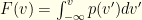Let’s examine the problem from a Bayesian perspective. There is a 50-50 chance that ${(z,z')=(x,y)}$ or ${(z,z')=(y,x)}$ . So ${p(z=x)=p(z=y)=0.5}$ . There are no subtleties lurking here. We’ve assumed nothing about the underlying distribution over ${(x,y)}$ . Whatever ${(x,y)}$ the envelopes contain, we are equally likely to initially pick the one with ${x}$ or the one with ${y}$ .

Once the initial envelope has been opened, and the value ${z}$ revealed, we sample ${d}$ from our selected distribution ${P}$ and clearly have ${p(d<x)=F(x)}$ and ${p(d<y)=F(y)}$ and ${p(d<z)=F(z)}$ . The latter forms the criterion by which we will keep ${z}$ or switch to ${z'}$ . Please note that in what follows, ${d}$ is not a free variable, but rather a mere notational convenience. Something like ${p(x<d)}$ is just notation for “the probability the sampled value is greater than ${x}$ .” We can apply Bayes’ law to get (with all probabilities conditional on some unknown choice of ${(x,y)}$ ):

$\displaystyle p(z=x|d<z)= \frac{p(d<z|z=x)p(z=x)}{p(d<z)}$

What we really care about is the ratio:

$\displaystyle \frac{p(z=x | d<z)}{p(z=y | d<z)}= \frac{p(d<z|z=x)p(z=x)}{p(d<z|z=y)p(z=y)}= \frac{F(x)}{F(y)}<1$

Here, we’ve observed that ${p(d<z|z=x)= p(d<x)= F(x)}$ and ${F(x)<F(y)}$ since by assumption ${x<y}$ and ${F}$ is monotonically increasing (we assumed its support is all of ${R}$ ). I.e., if ${d<z}$ there is a greater probability that ${z=y}$ than ${z=x}$ . We shouldn’t switch. A similar argument shows we should switch if ${d>z}$ .

So what the heck has happened, and where did the new information come from? What happened is that we actually know one piece of information we had not used: that the interval ${(x,y)}$ has nonzero probability measure. I.e. there is some “space” between ${x}$ and ${y}$ . We don’t know the underlying distribution but we can pretend we do. Our strategy will be worse than if we did know the underlying ${p(x)}$ , of course. We’ll return to this shortly, but first let’s revisit the assumptions which make this work. We don’t need the envelopes to contain real numbers, but we do require the following of the values in the envelopes:

The set of possible values forms a measurable set with a strict linear ordering.
Between any two elements there is a volume with nonzero probability. Actually, this only is necessary if we require a nonzero improvement for any ${(x,y)}$ . If we only require an improvement on average we don’t need it. But in that scenario, the host can contrive to use a distribution which neutralizes our strategy and returns us to 50-50 odds.

What difference does ${P}$ itself make? We don’t have any way to choose an “optimal” distribution because that would require placing the bulk of probability where we think ${x}$ and ${y}$ are likely to lie. I.e. we would require prior knowledge. All we can guarantee is that we can improve things by some (perhaps tiny) amount. We’ll compute how much (for a given true underlying distribution) shortly.

Let’s assume that ${Q(x,y)}$ is the true underlying distribution over ${(x,y)}$ . We won’t delve into what it means to “know” ${Q}$ since we are handed the envelopes to begin with. Perhaps the game is played many times with values drawn according to ${Q}$ or maybe it is a one-time affair with ${(x,y)}$ fixed (i.e. ${Q}$ a ${\delta}$ -distribution). Ultimately, such considerations just would divert us to the standard core philosophical questions of probability theory. Suffice to say that there exists some ${Q(x,y)}$ . By definition ${Q(x,y)=0}$ unless ${x<y}$ . For convenience, we’ll define a symmetrized version as well: ${q(a,b)\equiv Q(a,b)+Q(b,a)}$ . We don’t employ a factor of ${1/2}$ since the two terms are nonzero on disjoint domains.

Given ${Q}$ , what gain do we get from a particular choice of ${P}$ ?

$\displaystyle \begin{array}{rcl} P(win)= \int_{x<y} dx dy Q(x,y)[p(z=x|(x,y))p(x<d) \\ + p(z=y|(x,y))p(d<y)] \end{array}$

I.e., the probability we keep ${z}$ when it is ${y}$ and switch when it is ${x}$ . Clearly, ${p(z=x|(x,y))= p(z=y|(x,y))= 0.5}$ since those are the immutable 50-50 envelope ordering probabilities. After a little rearrangement, we get:

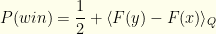
$\displaystyle P(win)= \frac{1}{2} + \langle F(y) - F(x) \rangle_Q$

Our gain is the mean value of ${F(y)-F(x)}$ over the joint distribution ${Q(x,y)}$ . The more probability ${P}$ jams between ${x}$ and ${y}$ , the more we gain should that ${(x,y)}$ arise. But without knowledge of the underlying joint distribution ${Q(x,y)}$ , we have no idea how best to pick ${P}$ . All we can do is guarantee some improvement.

How well can we do if we actually know ${Q}$ ? Well, there are two ways to use such information. We could stick to our strategy and try to pick an optimal ${P}$ , or we could seek to use knowledge of ${Q}$ directly. In order to do the former, we need to exercise a little care. ${Q}$ is a two-dimensional distribution while ${P}$ is one-dimensional. How would we use ${Q}$ to pick ${P}$ ? Well, this is where we make use of the observed ${z}$ .

In our previous discussion of the ${(x,2x)}$ envelope switching fallacy, the value of ${z}$ turned out to be a red-herring. Here it is not. Observing ${z}$ is essential here, but only for computation of probabilities. As mentioned, we assume no algebraic properties and are computing no expectations. We already know that the observation of ${z}$ is critical, since our algorithm pivots on a comparison between ${z}$ and our randomly sampled value ${d}$ . Considering our ultimate goal (keep or switch), it is clear what we need from ${Q}$ : a conditional probability that ${z'>z}$ . However, we cannot directly use ${Q(y|x)}$ because we defined ${x<y}$ . We want ${p(z'|z)}$ and we don’t know whether ${z<z'}$ or ${z'<z}$ . Let’s start by computing the probability of ${z}$ (being the observed value) and of ${z,z'}$ (being the observed and unobserved values).

The probability of observing ${z}$ and the other envelope having ${z'}$ is the probability that the relevant ordered pair was chosen for the two envelopes multiplied by the ${1/2}$ probability that we initially opened the envelop containing the value corresponding to our observed ${z}$ rather than the other one.

$\displaystyle p(z,z')= Q(min(z,z'),max(z,z'))/2= q(z,z')/2$

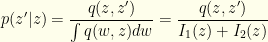
To get ${p(z)}$ we integrate this. ${p(z)= \frac{1}{2}\int Q(z,y)dy + \frac{1}{2}\int Q(x,z)dz}$ . This is a good point to introduce two quantities which will be quite useful going forward.

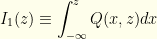
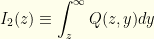
$\displaystyle I_1(z)\equiv \int_{-\infty}^z Q(x,z) dx$

$\displaystyle I_2(z)\equiv \int_z^\infty Q(z,y) dy$

In terms of these,

$\displaystyle p(z)= \frac{1}{2}[I_1(z)+I_2(z)]$

There’s nothing special about calling the variables ${x}$ or ${y}$ in the integrals and it is easy to see (since each only covers half the domain) that we get what we would expect:

$\displaystyle p(z)= \frac{1}{2}\int q(w,z)dw$

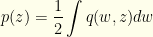
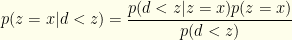
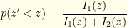
What we want is the distribution ${p(z'|z)= p(z,z'|z)= p(z,z')/p(z)= q(z,z')/p(z)}$ . This gives us:

$\displaystyle p(z'|z)= \frac{q(z,z')}{\int q(w,z)dw}= \frac{q(z,z')}{I_1(z)+I_2(z)}$

Finally, this gives us the desired quantity 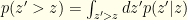${p(z'>z)= \int_{z'>z} dz' p(z'|z)}$ . It is easy to see that:

$\displaystyle p(z'<z)= \frac{I_1(z)}{I_1(z)+I_2(z)}$

$\displaystyle p(z'>z)= \frac{I_2(z)}{I_1(z)+I_2(z)}$

As an example, consider the previous ${(x,2x)}$ case — where one envelope holds twice what the other does. We observe ${z}$ , and ${z'}$ must be either ${2z}$ or ${z/2}$ , though we don’t know with what probabilities. If we are given the underlying distribution on ${x}$ , say ${P_2(x)}$ , we can figure that out. ${Q(x,y)= P_2(x)\delta(y-2x)}$ and ${q}$ is the symmetrized version. ${\int q(w,z)dw= \int dw [Q(w,z)+Q(z,w)]= (P_2(z/2)+P_2(2z))}$ . So ${p(z)= \frac{1}{2}(P_2(z/2)+P_2(2z))}$ . This is just what we’d expect — though we’re really dealing with discrete values and are being sloppy (which ends us up with a ratio of infinities from the ${\delta}$ function when computing probability ratios, but we’ll ignore that here). The relevant probability ratio clearly is 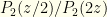${P_2(z/2)/P_2(2z)}$ . From a purely probability standpoint, we should switch if 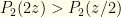${P_2(2z)>P_2(z/2)}$ . If we reimpose the algebraic structure and try to compute expectations (as in the previous problem) we would get an expected value of ${z}$ from keeping and an expected value of ${z[P_2(z/2)/2 + 2P(2z)]}$ from switching . Whether this is less than or greater than ${z}$ depends on the distribution ${P_2}$ .

Returning to our analysis, let’s see how often we are right about switching if we know the actual distribution ${Q}$ and use that knowledge directly. The strategy is obvious. Using our above formulae, we can compute ${p(z'<z)}$ directly. To optimize our probability of winning, we observe ${z}$ then we switch iff ${I_1(z)<I_2(z)}$ . If there is additional algebraic structure and expectations can be defined, then an analogous calculations give whatever switching criterion maximizes the relevant expectation value.

In terms of probabilities, full knowledge of ${Q}$ is the best we can do. The probability we act correctly is:

$\displaystyle \begin{array}{rcl} P'(win)= \int dz \frac{[\theta(I_1(z)-I_2(z)) I_1(z) + \theta(I_2(z)-I_1(z))I_2(z)]}{I_1(z)+I_2(z)} \\ = \int dz \frac{\max(I_1(z),I_2(z))}{(I_1(z)+I_2(z)} \end{array}$

$\displaystyle P'(win|z)= \frac{\max(I_1(z),I_2(z))}{(I_1(z)+I_2(z)}$

Since ${I_1}$ and ${I_2}$ are monotonic (one increasing, the other decreasing), we have a cutoff value ${\hat z}$ (defined by ${I_1({\hat z})= I_2({\hat z})}$ ) below which we should switch and above which we should not.

How do we do with our invented ${P}$ instead? We could recast our earlier formula for ${P(win)}$ into our current notation, but it’s easier to compute directly. For given ${z}$ , the actual probability of needing to switch is 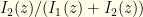${I_2(z)/(I_1(z)+I_2(z))}$ . Based on our algorithm, we will do so with probability 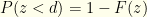${P(z<d)= 1-F(z)}$ . The probability of not needing to switch is ${I_1(z)}$ and we do so with probability 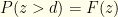${P(z>d)= F(z)}$ . I.e., our probability of success for given ${z}$ is:

$\displaystyle P(win|z)= \frac{I_1(z)F(z) + I_2(z)(1-F(z))}{I_1(z)+I_2(z)}$

For any given ${z}$ , this is of the form ${\alpha r + (1-\alpha)(1-r)}$ where ${r= F(z)}$ and ${\alpha= I_1(z)/(I_1(z)+I_2(z))}$ . The optimal solutions lie at one end or the other. So it obviously is best to have ${F(z)=0}$ when ${z<{\hat z}}$ and ${F(z)=1}$ when ${z>{\hat z}}$ . This would be discontinuous, but we could come up with a smoothed step function (ex. a logistic function) which is differentiable but arbitrarily sharp. The gist is that we want all the probability in ${F}$ concentrated around ${\hat z}$ . Unfortunately, we have no idea where ${\hat z}$ is!

Out of curiosity, what if we pick instead ${P}$ to be the conditional distribution ${p(z'|z)}$ itself once we’ve observed ${z}$ ? We’ll necessarily do worse than by direct comparison using ${Q}$ (the max formula above), but how much worse? Well, ${p(z'|z)= q(z,z')/(I_1(z)+I_2(z))}$ . Integrating over ${z'<z}$ we have ${F(z)= \int_{-\infty}^z p(z'|z) dz'= I_1(z)/(I_1(z),I_2(z))}$ . I.e., We end up with ${(I_1^2(z)+I_2^2(z))/(I_1(z)+I_2(z))^2}$ as our probability of success. If we had used ${1-p(z'|z)}$ for our ${P}$ instead we would get ${2I_1(z)I_2(z)/(I_1(z)+I_2(z))^2}$ instead. Neither is optimal in general.

Next, let’s look at the problem from an information theory standpoint. As mentioned, there are two sources of entropy: (1) the choice of the underlying pair ${(x,y)}$ (with ${x<y}$ by definition) and (2) the selection ${(z,z')=(x,y)}$ or ${(z,z')=(y,x)}$ determined by our initial choice of an envelope. The latter is a fair coin toss with no information and maximum entropy. The information content of the former depends on the (true) underlying distribrution.

Suppose we have perfect knowledge of the underlying distribution. Then any given ${z}$ arises with probability ${p(z)=\frac{1}{2}[I_1(z)+I_2(z)]}$ . Given that ${z}$ , we have a Bernoulli random variable ${p(z'>z)}$ given by ${I_2(z)/(I_1(z)+I_2(z))}$ . The entropy of that specific coin toss (i.e. the conditional entropy of the Bernoulli distribution ${p(z'> z|z)}$ ) is

$\displaystyle H(z'>z|z)= \frac{-I_1(z)\ln I(z) - I_2(z)\ln I_2(z) + (I_1(z)+I_2(z))\ln [I_1(z)+I_2(z)]}{I_1(z)+I_2(z)}$

With our contrived distribution ${P}$ , we are implicitly are operating as if ${p(z'>z)= 1-F(z)}$ . This yields a conditional entropy:

$\displaystyle H'(z'>z|z)= -(1-F(z))\ln (1-F(z)) - F(z)\ln F(z)$

There is a natural measure of the information cost of assuming an incorrect distribution. It is the Kullback Liebler Divergence (also known as the relative entropy). While it wouldn’t make sense to compute it between ${Q}$ and ${P}$ (which are, among other things, of different dimension, we certainly can compare the cost for given ${z}$ of the difference in our Bernoulli random variables for switching — and then integrate over ${z}$ to get an average cost in bits. Let’s denote by ${q(z'>z)}$ the probability based on the true distribution and keep ${p(z'>z)}$ for the contrived one. I.e. ${q(z'>z)= I_2(z)/(I_1(z)+I_2(z))}$ and ${p(z'>z)= 1-F(z)}$ . For given ${z}$ , the K-L divergence is:

$\displaystyle D(Q || P, z)= \frac{-I_2(z)\ln [(I_1(z)+I_2(z))(1-F(z))/I_2(z)] - I_1(z)\ln [(I_1(z)+I_2(z))F(z)/I_1(z)]}{I_1(z)+I_2(z)}$

Integrating this, we get the mean cost in bits of being wrong.

$\displaystyle \begin{array}{rcl} \langle D(Q || P) \rangle= \frac{1}{2}\int dz [-(I_1(z)+I_2(z))\ln [I_1(z)+I_2(z)] - I_2(z)\ln (1-F(z)) \\ -I_1(z)\ln F(z) + I_1(z)\ln I_1(z) + I_2(z)\ln I_2(z)] \end{array}$

The first term is simply ${H(z)}$ , the entropy of our actual distribution over ${z}$ . In fact, the first term and last 2 terms together we recognize as ${\langle H(z'>z|z) \rangle}$ , the mean Bernoulli entropy of the actual distribution. In these terms, we have:

$\displaystyle \langle D(Q || P) \rangle= \langle H(z'>z|z) \rangle + \langle \frac{ -I_2(z)\ln(1-F(z)) - I_1(z)\ln F(z)}{I_1(z)+I_2(z)} \rangle$

where the expectations are over the unconditional actual distribution ${p(z)}$ . The 2nd expectation on the right represents the cost of being wrong about ${P}$ . If it was the optimal distribution with all probability centered near ${\hat z}$ then the term on the right would approach ${0}$ and there would be no entropy cost.

As an aside, this sort of probabilistic strategy should not be confused with the mixed strategies of game theory. In our case, a mixed strategy would be an apriori choice ${aK+(1-a)S}$ where ${K}$ is the always-keep strategy, ${S}$ is the always-switch strategy, and ${0\le a\le 1}$ is the probability of employing the always-keep strategy. A player would flip a biased-coin with Bernoulli probability ${a}$ and choose one of the two-strategies based on it. That has nothing to do with the measure-theory approach we’re taking here. In particular, a mixes strategy makes no use of the observed value ${x}$ or its relation to the randomly sampled value. Any mixed strategy gives even-odds because the two underlying deterministic strategies both have even-odds.

Musing, Research

A Travel-Time Metric

July 1, 2015 K.M. Halpern

Especially in urban areas, two locations may be quite close geographically but difficult to travel between. I wondered whether one could create a map where, instead of physical distances, points are arranged according to some sort of travel-time between them. This would be useful for many purposes.

Unfortunately, such a mapping is mathematically impossible in general (for topological reasons). But so is a true map of the Earth, hence the need for Mercator or other projections. The first step in constructing a useful visualization is to define an appropriate Travel-Time metric function. Navigation systems frequently compute point-to-point values, but they are not bound by the need to maintain a consistent set of Travel Times between all points. That is our challenge – to construct a Travel-Time metric.

Read the Paper (PDF)

Musing, Research

Inflation, Up Close and Personal

January 18, 2013 K.M. Halpern

It often seems like the inflation figures touted by officials and economists have little connection with the real world. There are a number of reasons for this, some technical and some political. But there is a deeper problem than the means and motives for calculating any specific index. The issue is that any aggregate number is likely to deviate significantly from one’s personal experience. Each of us saves for different reasons and spends in different ways. Without taking these specific choices into account, we cannot accurately represent or protect against the inflation that we individually encounter. This paper elaborates on this idea and explains how each of us can identify the relevant components of inflation, and best hedge our savings.

Read the Paper (PDF)

Musing, Research

Probabilistic Sentencing

February 10, 2012 K.M. Halpern

In most real situations, we must make decisions based on partial information. We should neither allow this uncertainty to prevent action or pretend to perfect certainty in taking action. Yet in one area with a great impact on an individual’s freedom and well-being we do just that. Judges and juries are required to return an all-or-nothing verdict of guilt. They may not use their experience, intelligence, and judgment to render a level of confidence rather than a mere binary choice.

I propose adopting a sentencing mechanism based on a probabilistic assessment of guilt or innocence. This allows jurists to better express their certainty or lack thereof than does our traditional all-or-nothing verdict. The natural place to reflect such an imputed degree of guilt is in the sentencing phase. I discuss the implications of such a system as well as certain issues with implementation.

Read the Paper (PDF)

Musing, Research

A System for Fairness in Sentencing

February 7, 2012 K.M. Halpern

We often hear of cases that offend our sense of fairness – excessive sentences, minor crimes that are punished more severely than serious crimes, or two equivalent crimes that are punished very differently. Rather than attempt to solve a politically and legally intractable problem, we ask a more theoretical question: whether an individual can assign sentences in a way that seems reasonable and consistent to him. Our system is a means of doing so. We offer a simple algorithmic method that could be used by an individual or review board to ensure that sentences meet a common-sense standard of consistency and proportionality.

We intend to offer a less mathematical and more legally-oriented version of this article in the near future.

Read the Paper (PDF)

knotes, Notes

Differential Entropy

January 31, 2012 K.M. Halpern

A discussion of some of the subtleties of differential entropy. This also contains a review of discrete entropy, various entropy-related information quantities such as mutual information, and a listing of various axiomatic formulations.

Read the Notes (PDF)

Musing

The Optics of Camera Lens Stacks (Program)

August 27, 2011 K.M. Halpern

In another post, I discussed the mathematical calculation of optical parameters for a configuration of stacked lenses and camera components. As is evident from the example worked out there, the procedure is somewhat tedious. Instead, it is better to spend twice the time writing a program to do it. Fortunately I already did this and offer it to you, gentle reader, to use and criticize. I expect no less than one rabid rant about some aspect that doesn’t pedantically conform to the IEEE standard. This is working code (and has been checked over and tested to some extent). I use it. However, it is not commercial grade and was not designed with either efficiency or robustness in mind. It is quick and dirty – but graciously so.

Think of this as a mine-shaft. You enter at your own risk and by grace of the owner. And if you fall, there won’t be non-stop human interest coverage on 20 TV channels as rescue workers try to extract you. That’s because you’re not a telegenic little kid and this is a metaphor. Rather, you will end up covered in numeric slime of dubious origin. But I still won’t care.

All this said, I do appreciate constructive criticism and suggestions. Please let me know about any bugs. I don’t plan to extensively maintain this program, but I will issue fixes for significant bugs.

The program I provide is a command line unix (including MacOS) utility. It should be quite portable, as no funky libraries are involved. The program can analyze a single user-specified configuration or scan over all possible configurations from an inventory file. In the latter case, it may restrict itself to configurations accessible using the included adapters or regardless of adapter. It also may apply a filter to limit the output to “interesting” cases such as very high magnification, very wide angle, or high telephoto.

The number of configurations can be quite large, particularly when many components are available, there are no constraints, and we account for the large number of focal/zoom choices for each given stack. For this reason, it is best to constrain scans to a few components in an inventory (by commenting out the components you don’t need). For example, if one has both 10 and 25mm extension tubes then try with only one. If this looks promising, restrict yourself to the components involved and uncomment the 25mm as well.

Either through the summary option or the use of a script to select out desirable configurations, the output may be analyzed and used for practical decisions. For example, if a 10x macro lens is needed and light isn’t an issue then a 1.4X telextender followed by a 200mm zoom followed by a reversed 28mm will do the trick. It will have a high f-stop, but if those components are already owned and we don’t need a low f-stop it may be far more cost-effective option than a dedicated ultra-macro lens (there aren’t any at 10X, but a 5X one is available).

For simple viewing of the results, I recommend the use of my “tless” utility. This isn’t a shameless plug. I wrote tless for myself, and I use it extensively.

Go to Google Code Archive for Project

Musing, Notes

The Optics of Camera Lens Stacks (Analysis)

August 24, 2011 K.M. Halpern

This first appeared on my tech blog. I like to play around with various configurations of camera lenses. This partly is because I prefer to save money by using existing lenses where possible, and partly because I have a neurological condition (no doubt with some fancy name in the DSM-IV) that compels me to try to figure things out. I spent 5 years at an institute because of this problem and eventually got dumped on the street with nothing but a PhD in my pocket. So let this be a warning: keep your problem secret and don’t seek help.

A typical DSLR (or SLR) owner has a variety of lenses. Stacking these in various ways can achieve interesting effects, simulate expensive lenses (which may internally be similar to such a stack), or obtain very high magnifications. Using 3 or 4 lenses, a telextender, a closeup lens, and maybe some extension rings (along with whatever inexpensive adapter rings are needed), a wide variety of combinations can be constructed. In another entry, I’ll offer a companion piece of freeware that enumerates the possible configurations and computes their optical properties.

In the present piece, I examine the theory behind the determination of those properties for any particular setup. Given a set of components (possibly reversed) and some readily available information about them and the camera, we deduce appropriate optical matrices, construct an effective matrix for the system, and extract the overall optical properties – such as focal length, nearest object distance, and maximum magnification. We account for focal play and zoom ranges as needed.

The exposition is self-contained, although this is not a course on optics and I simply list basic results. Rather, I focus on the application of matrix optics to real camera lenses. I also include a detailed example of a calculation.

As far as I am aware, this is the only treatment of its kind. Many articles discuss matrix methods or the practical aspects of reversing lenses for macro photography. However, I have yet to come across a discussion of how to deduce the matrix for a camera lens and vice-versa.

After reading the piece, you may wonder whether it is worth the effort to perform such a calculation. Wouldn’t it be easier to simply try the configurations? To modify the common adage, a month on the computer can often save an hour in the lab. The short answer is yes and no. No I’m not an economist, why do you ask?

If you have a specific configuration in mind, then trying it is easier. However, if you have a set of components and want to determine which of the hundreds of possible configurations are candidates for a given use (just because the calculation works, doesn’t mean the optical quality is decent), or which additional components one could buy to make best use of each dollar, or which adapter rings are needed, or what end of the focal ranges to use, then the calculation is helpful. Do I recommend doing it by hand? No. I even used a perl script to generate the results for the example. As mentioned, a freeware program to accomplish this task in a more robust manner will be forthcoming. Think of the present piece as the technical manual for it.

Read the Paper (PDF)

knotes, Notes

Cardinality

August 2, 2011 K.M. Halpern

A compilation of useful results involving cardinal numbers (small ones, not huge ones) and arithmetic, along with the cardinalities of certain useful sets. There’s also a small section on bases of infinite-dimensional vector spaces. Proofs and justifications for many of the results are included in an appendix.

Read the Paper

Musing, Research

Influence in Voting

April 30, 2008 K.M. Halpern

Have you ever wondered what really is meant by a “deciding vote” on the Supreme Court or a “swing State” in a presidential election? These terms are bandied about by the media, but their meaning isn’t obvious. After all, every vote is equal, isn’t it? I decided to explore this question back in 2004 during the election year media bombardment. What started as a simple inquiry quickly grew into a substantial project. The result was an article on the subject, which I feel codifies the desired understanding. The paper contains a rigorous mathematical framework for block voting systems (such as the electoral college), a definition of “influence”, and a statistical analysis of the majority of elections through 2004. The work is original, but not necessarily novel. Most if not all has probably been accomplished in the existing literature on voting theory. This said, it may be of interest to a technical individual interested in the subject. It is self-contained, complete, and written from the standpoint of a non-expert in the field. For those who wish to go further, my definition of “influence” is related to the concept of “voting power” in the literature (though I am unaware of any analogue to my statistical definition).

Read the Paper (PDF)

Musing, Research

Ye Olde Physics Papers

June 2, 1998 K.M. Halpern

Once upon a time there was a physicist. He was productive and happy and dwelt in a land filled with improbably proportioned and overly cheerful forest creatures. Then a great famine of funding occurred and the dark forces of string theory took power and he was cast forth into the wild as a heretic. There he fought megalomaniacs and bureaucracies and had many grand adventures that appear strangely inconsistent on close inspection. The hero that emerged has the substance of legend.

But back to me. I experienced a similar situation as a young physicist, but in modern English and without the hero bit. However, once upon a time I DID write physics papers. This is their story…

My research was in an area called Renormalization Group theory (for those familiar with the subject, that’s the “momentum-space” RG of Quantum Field Theory, rather than the position-space version commonly employed in Statistical Mechanics – although the two are closely related).

In simple terms, one could describe the state of modern physics (then and now) as centering around two major theories: the Standard Model of particle physics, which describes the microscopic behavior of the electromagnetic, weak, and strong forces, and General Relativity, which describes the large scale behavior of gravity. These theories explain all applicable evidence to date, and no prediction they make has been excluded by observation (though almost all our effort has focused on a particular class of experiment, so this may not be as impressive as it seems). In this sense, they are complete and correct. However, they are unsatisfactory.

Their shortcomings are embodied in two of the major problems of modern physics (then and now): the origin of the Standard Model and a unification of Quantum Field Theory with General Relativity (Quantum Field Theory itself is the unification of Quantum Mechanics with Special Relativity). My focus was on the former problem.

The Standard Model is not philosophically satisfying. Besides the Higgs particle, which is a critical component but has yet to be discovered, there is a deeper issue. The Standard Model involves a large number of empirical inputs (about 21, depending on how you count them), such as the masses of leptons and quarks, various coupling constants, and so on. It also involves a specific non-trivial set of gauge groups, and doesn’t really unify the strong force and electro-weak force (which is a proper unification of the electromagnetic and weak forces). Instead, they’re just kind of slapped together. In this sense, it’s too arbitrary. We’d like to derive the entire thing from simple assumptions about the universe and maybe one energy scale.

There have been various attempts at this. Our approach was to look for a “fixed point”. By studying which theories are consistent as we include higher and higher energies, we hoped to narrow the field from really really big to less really really big – where “less really really big” is 1. My thesis and papers were a first shot at this, using a simple version of Quantum Field Theory called scalar field theory (which coincidentally is useful in it’s own right, as the Higgs particle is a scalar particle). We came up with some interesting results before the aforementioned cataclysms led to my exile into finance.

Unfortunately, because of the vagaries of copyright law I’m not allowed to include my actual papers. But I can include links. The papers were published in Physical Review D and Physical Review Letters. When you choose to build upon this Earth Shattering work, be sure to cite those. They also appeared on the LANL preprint server, which provides free access to their contents. Finally, my thesis itself is available. Anyone can view it, but only MIT community members can download or print it. Naturally, signed editions are worth well into 12 figures. So print and sign one right away.

First Paper on LANL (free content)
Second Paper on LANL (free content)
Third Paper on LANL (free content)
First Paper on Spires
Second Paper on Spires
Third Paper on Spires
Link to my Thesis at MIT

A Place of Sand

Tag Archives: mathy

Semidirect Products, Group Extensions, Split Exact Sequences, and all that

What happens when you iterate Bayesian Inference with the same data set?

CCSearch State Space Algo

Two-Envelope Problems

A Travel-Time Metric

Inflation, Up Close and Personal

Probabilistic Sentencing

A System for Fairness in Sentencing

Differential Entropy

The Optics of Camera Lens Stacks (Program)

The Optics of Camera Lens Stacks (Analysis)

Cardinality

Influence in Voting

Ye Olde Physics Papers

Writings and Ravings